Nedenfor er alle illustrationerne og data-plottene jeg har lavet til afhandlingen.
I figurteksten for hver kan du også finde download links direkte til figurerne enten i 900 dpi PNG (og nogle gange med en transparent bagground, vist som αPNG) eller vektorformat (SVG og PDF), samt links til andre relevante versioner af figurerne.
De fleste af illustrationerne er lavet i LaTeX ved hjælp af PSTricks, mens de fleste dataplots er lavet i enten MATLAB eller ved brug af Python.
Nogle af dem blev oprindeligt lavet til mit kandidatspeciale, dog med opdateringer til PhD afhandlingen.
Superlednings-illustrationer (kapitel 2)
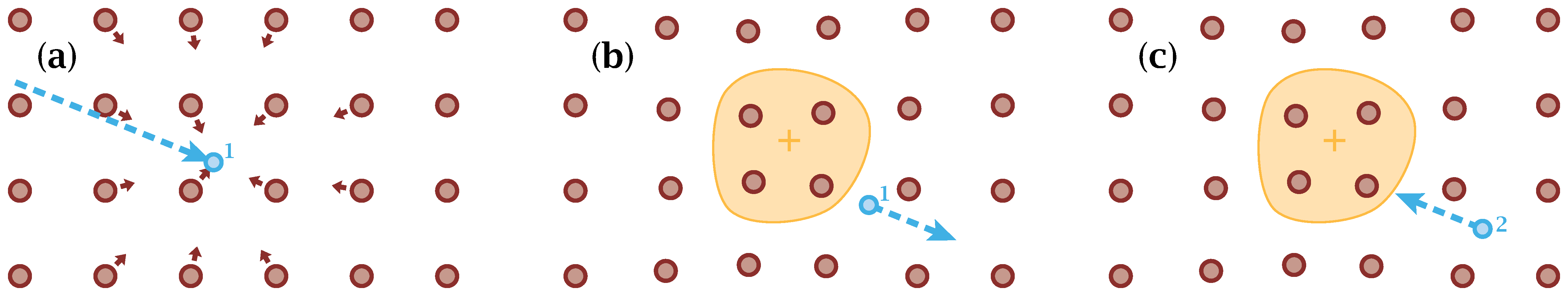
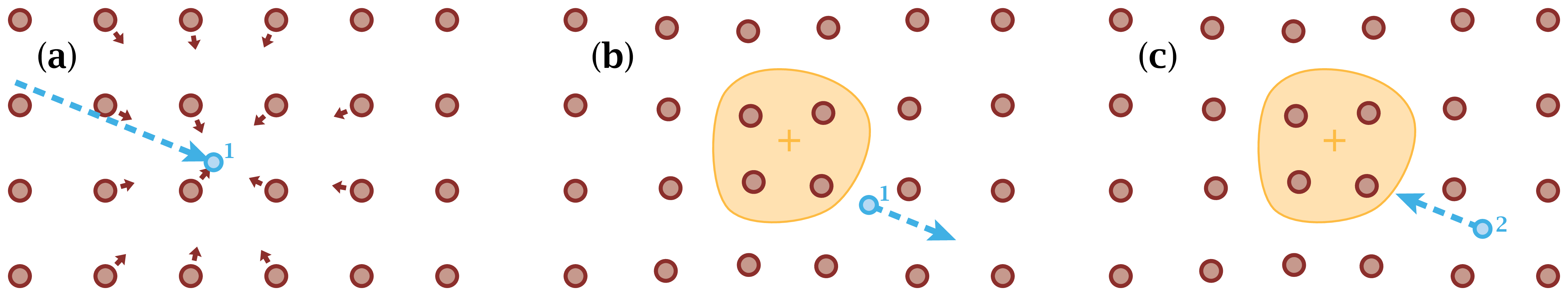
Figur 2.1: Mediation of a bosonic pair of electrons via phonons. Download links:PNG • αPNG • SVG • PDF. .
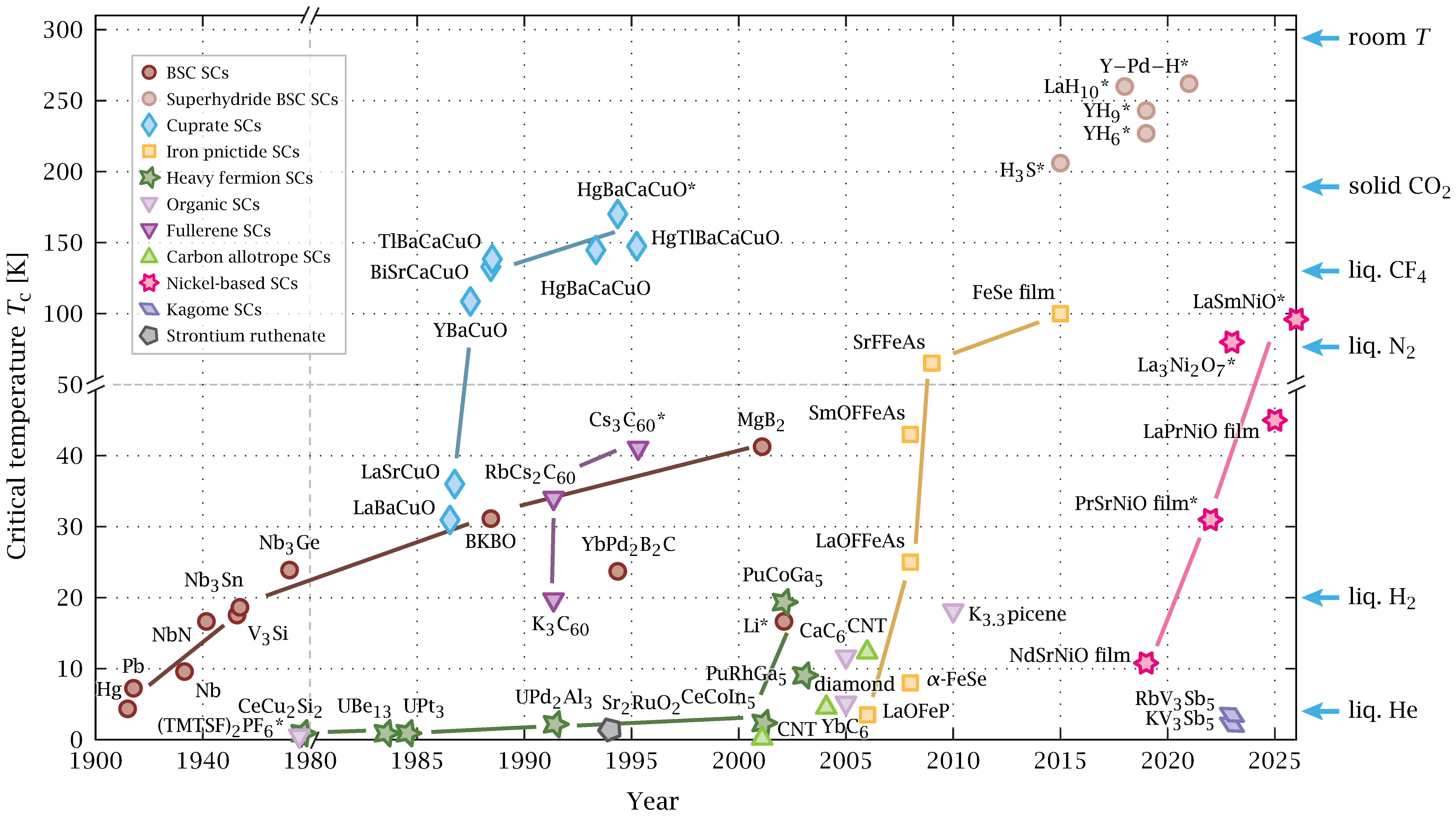
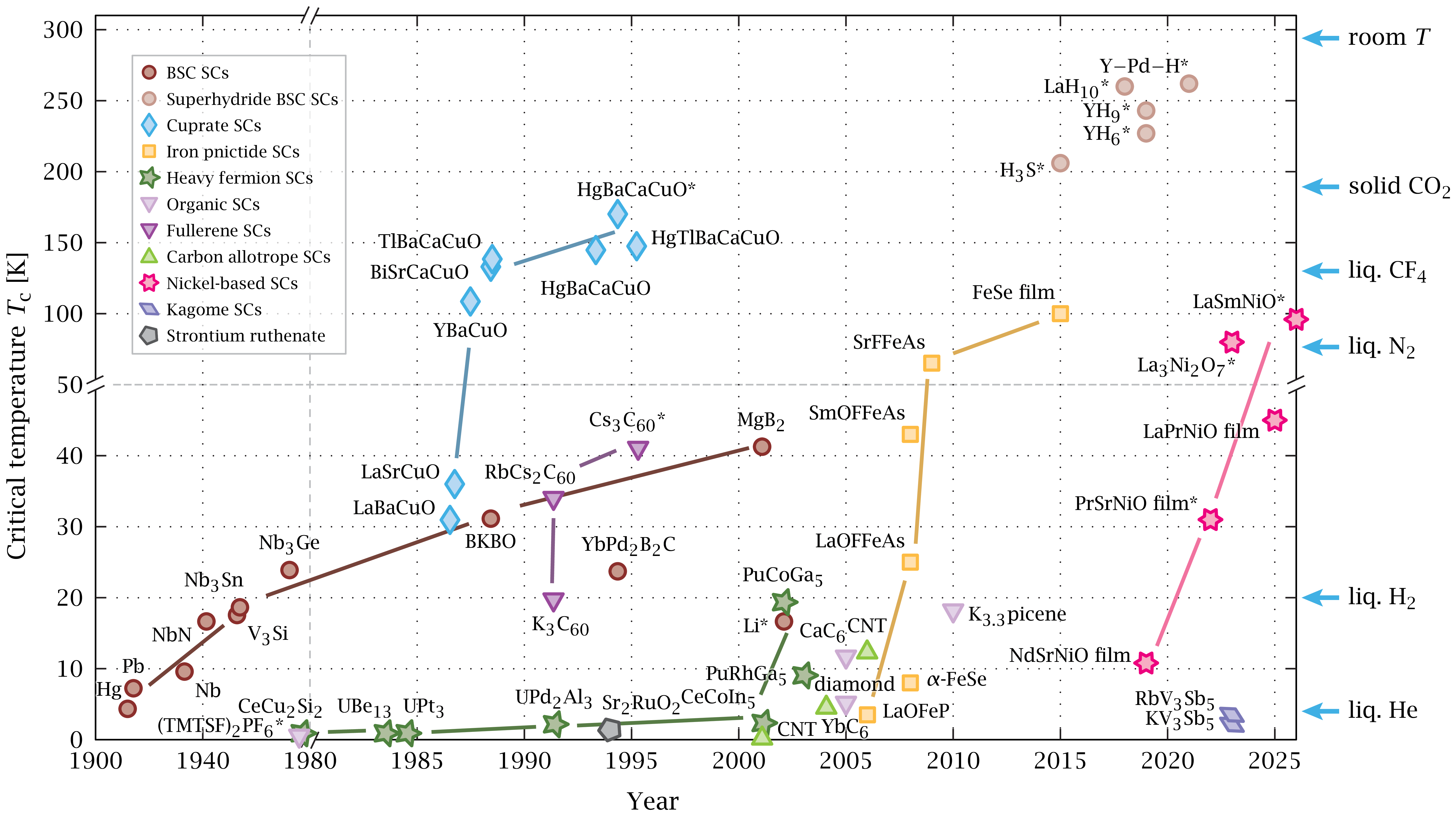
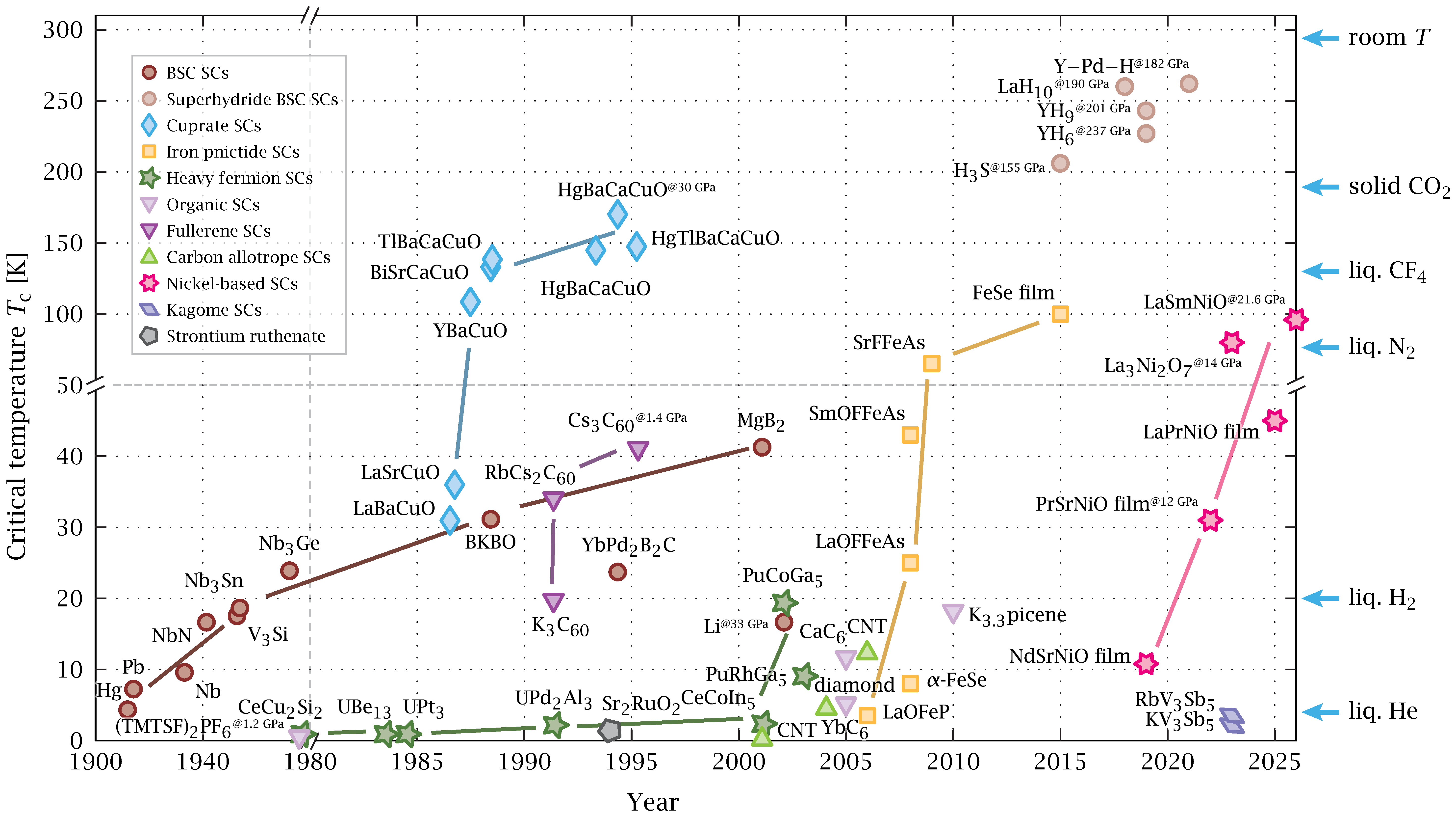
Figur 2.2: Timeline for the history of superconducting compounds. Download links:PNG • αPNG • SVG • PDF. Second version with the pressures shown as values: PNG•αPNG•SVG•PDF.
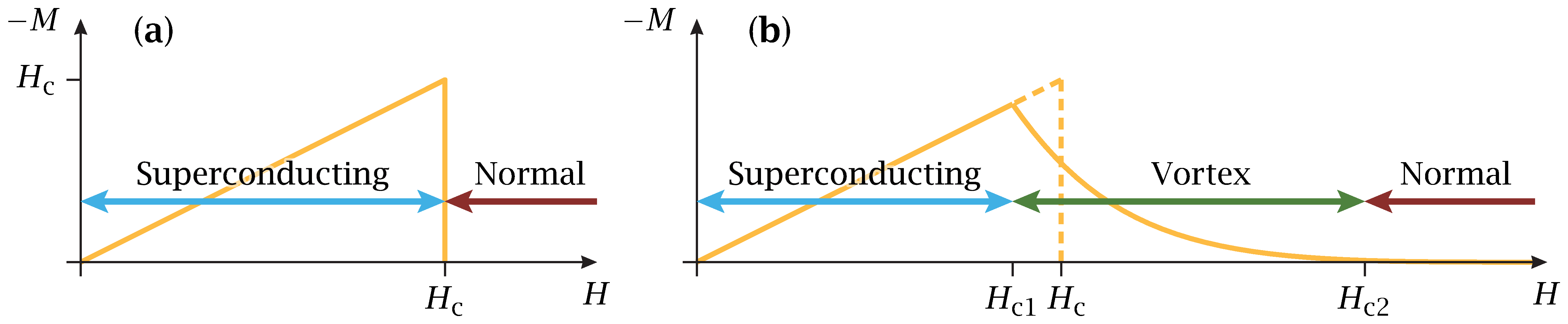
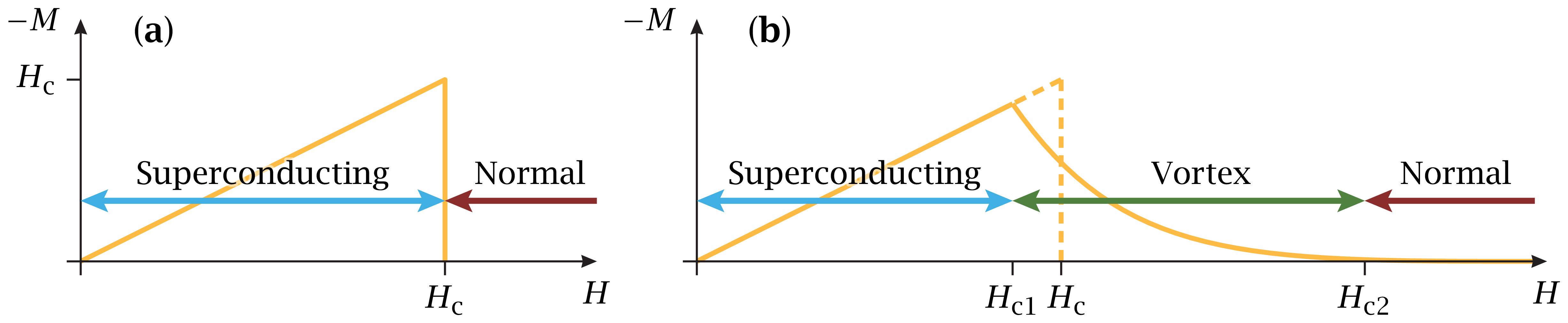
Figur 2.3: The magnetisation of a superconductor as a function of applied field. Download links:PNG • αPNG • SVG • PDF. .
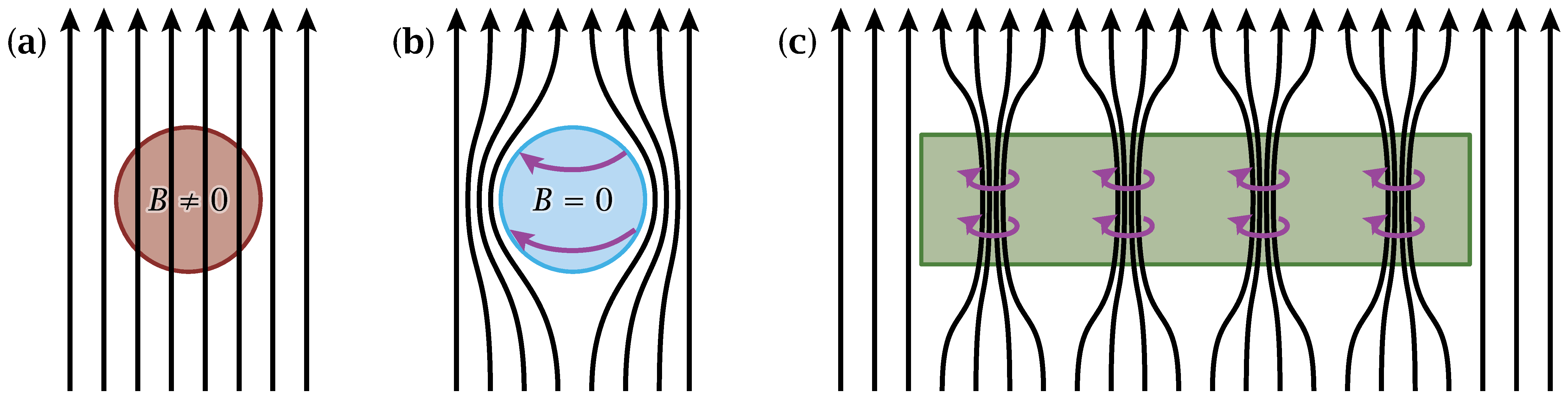
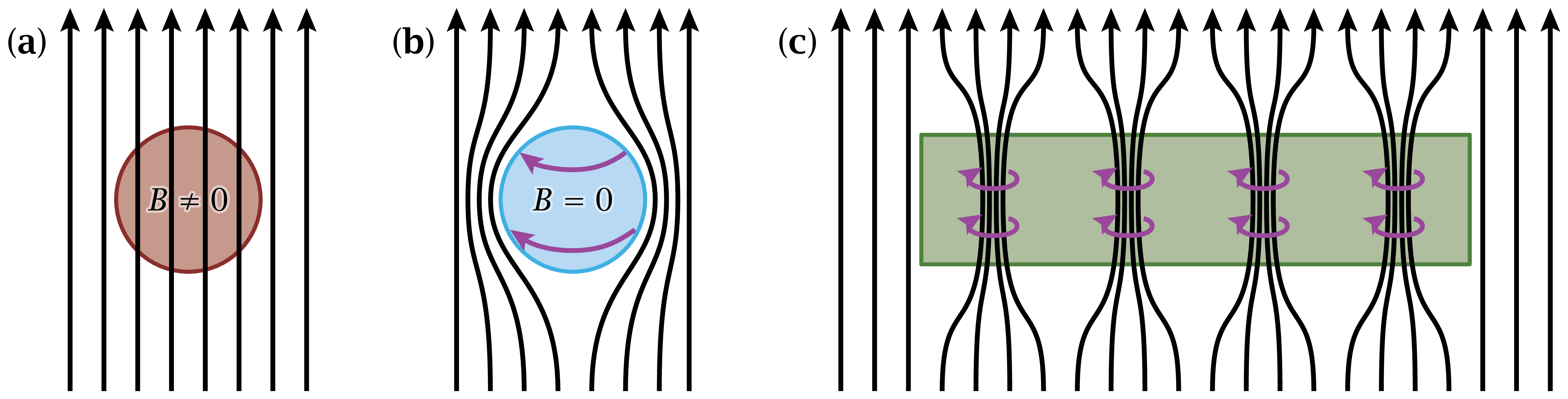
Figur 2.4: Magnetic field lines for a superconductor. Download links:PNG • αPNG • SVG • PDF. .
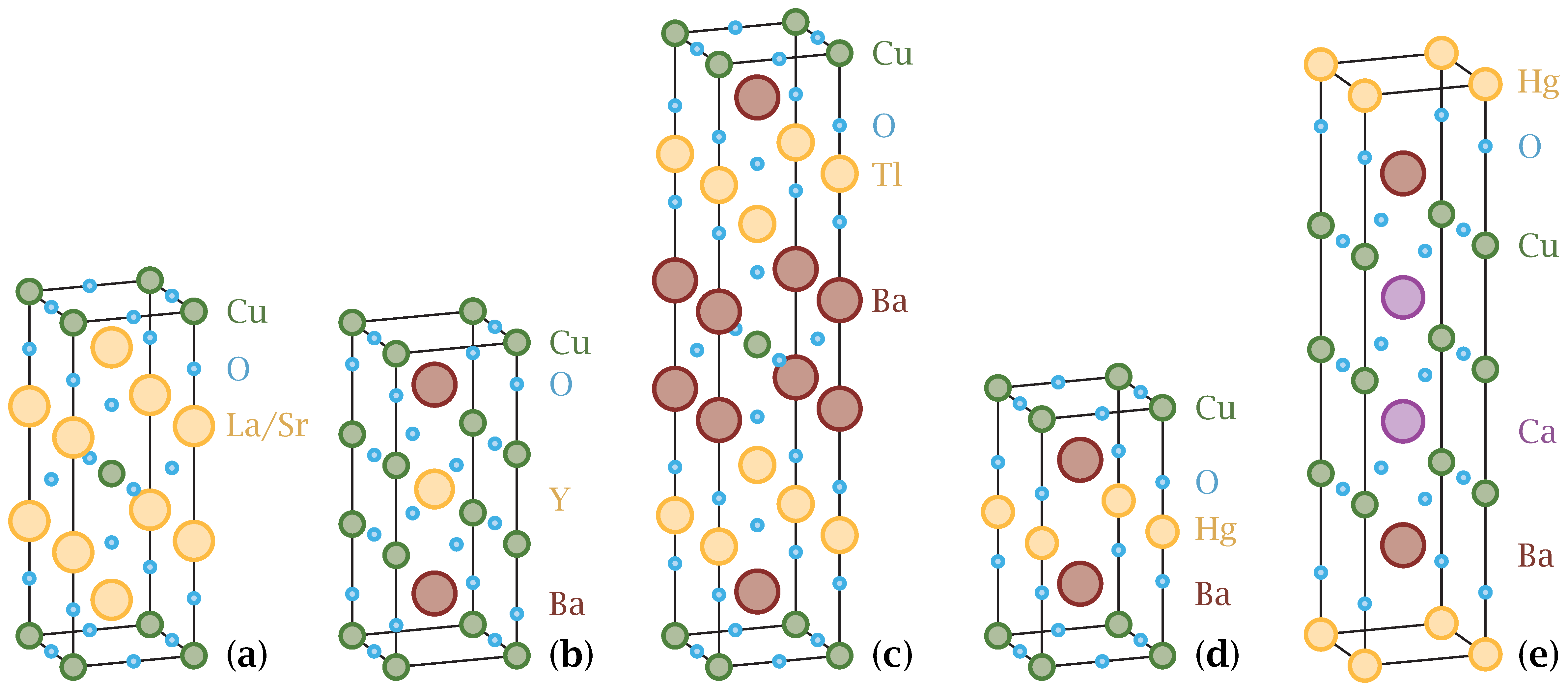
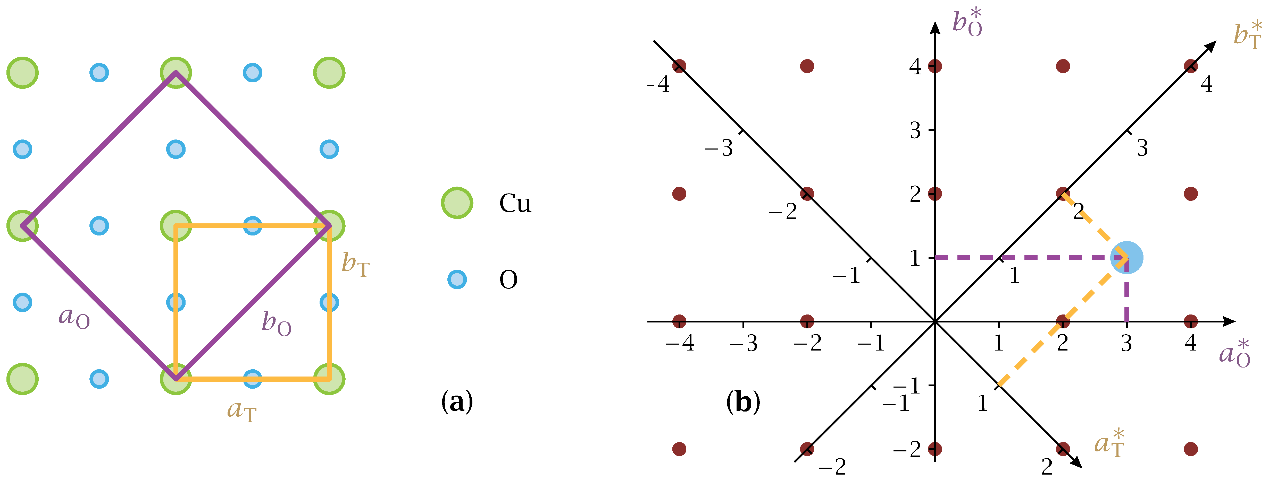
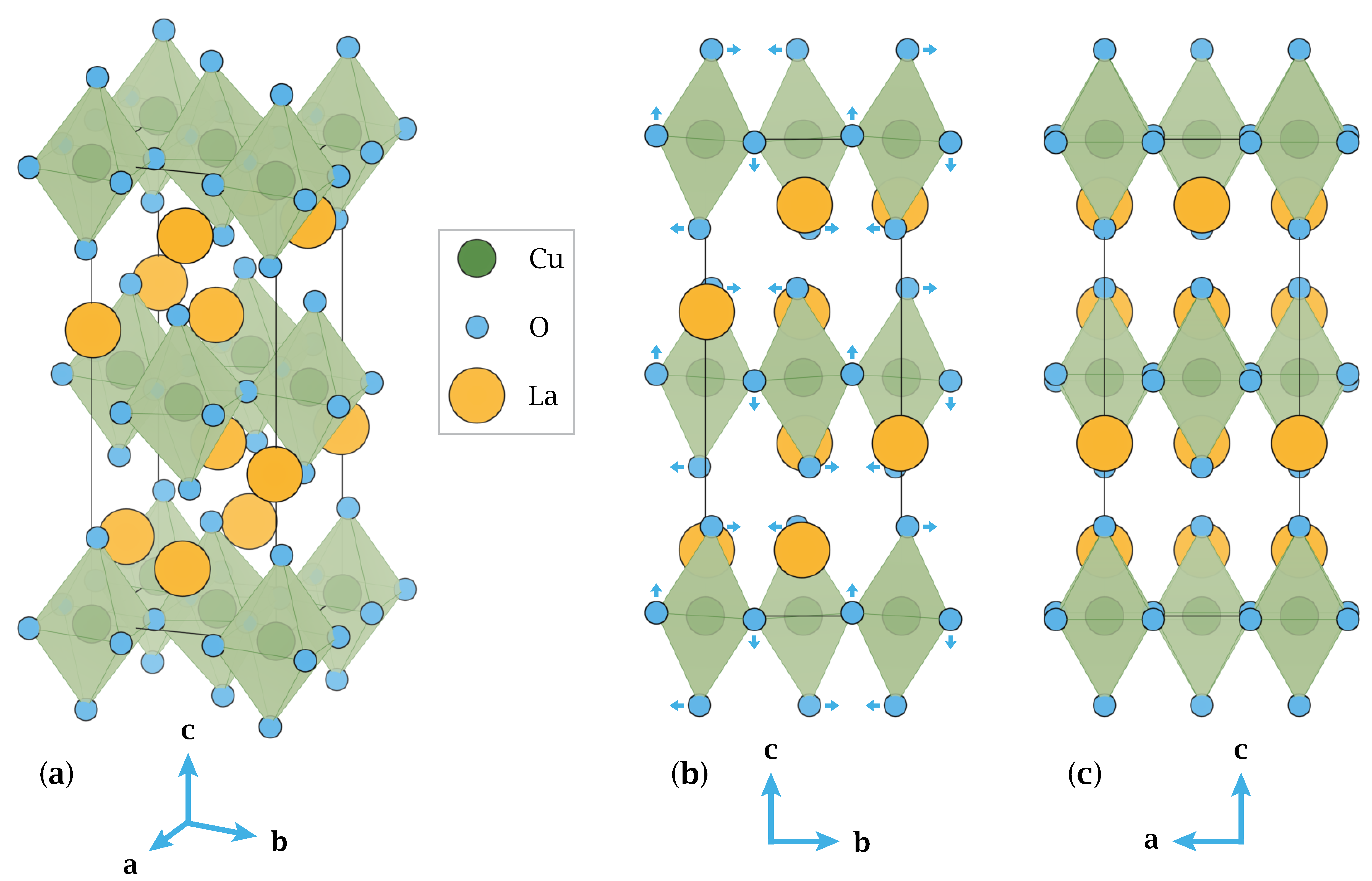
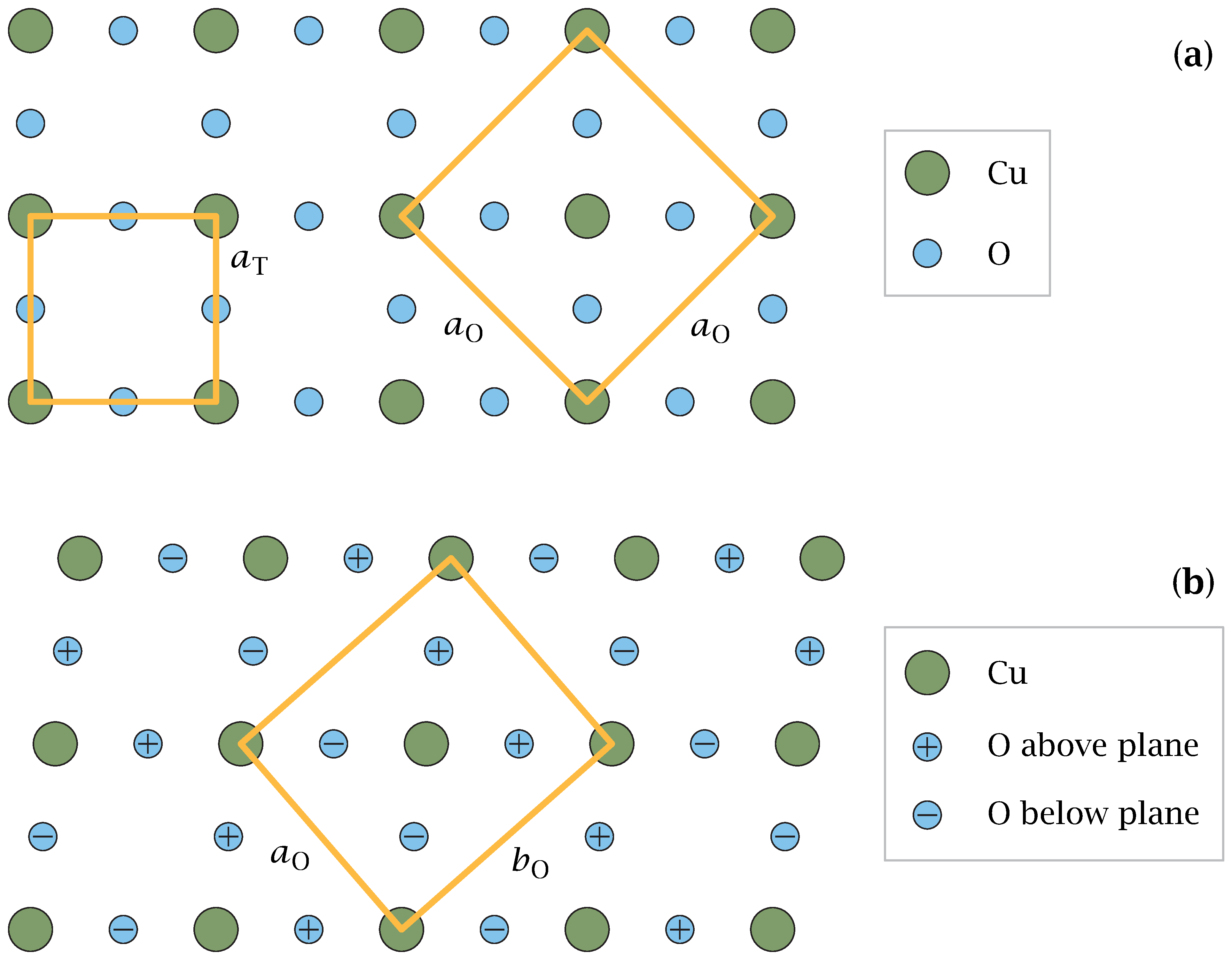
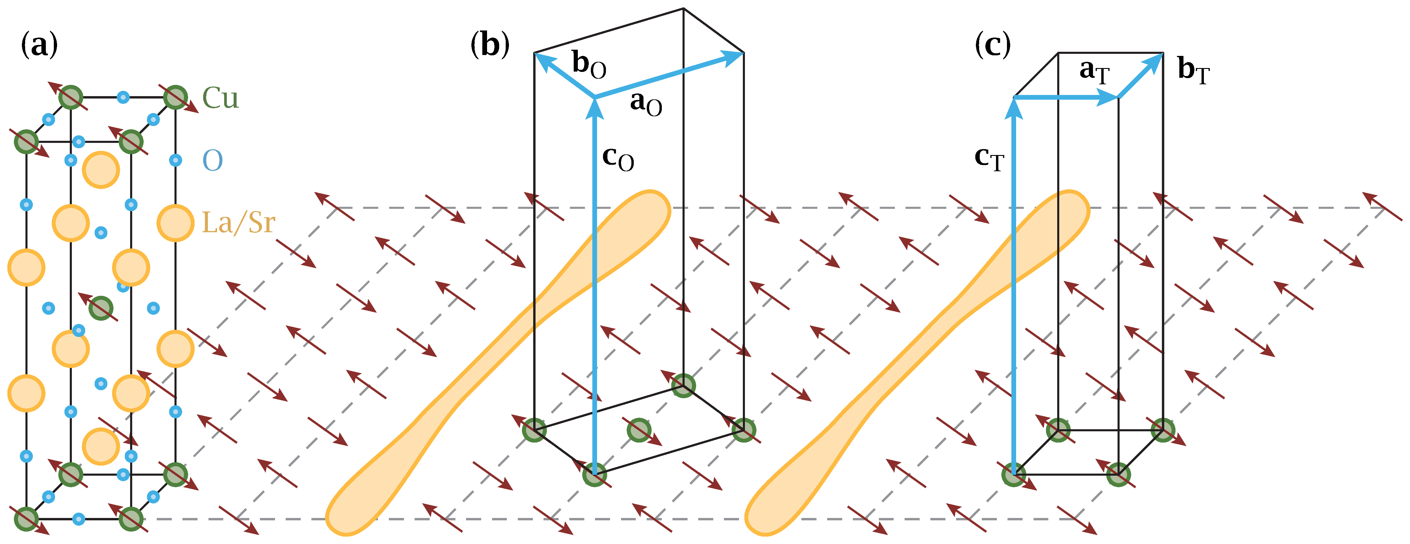
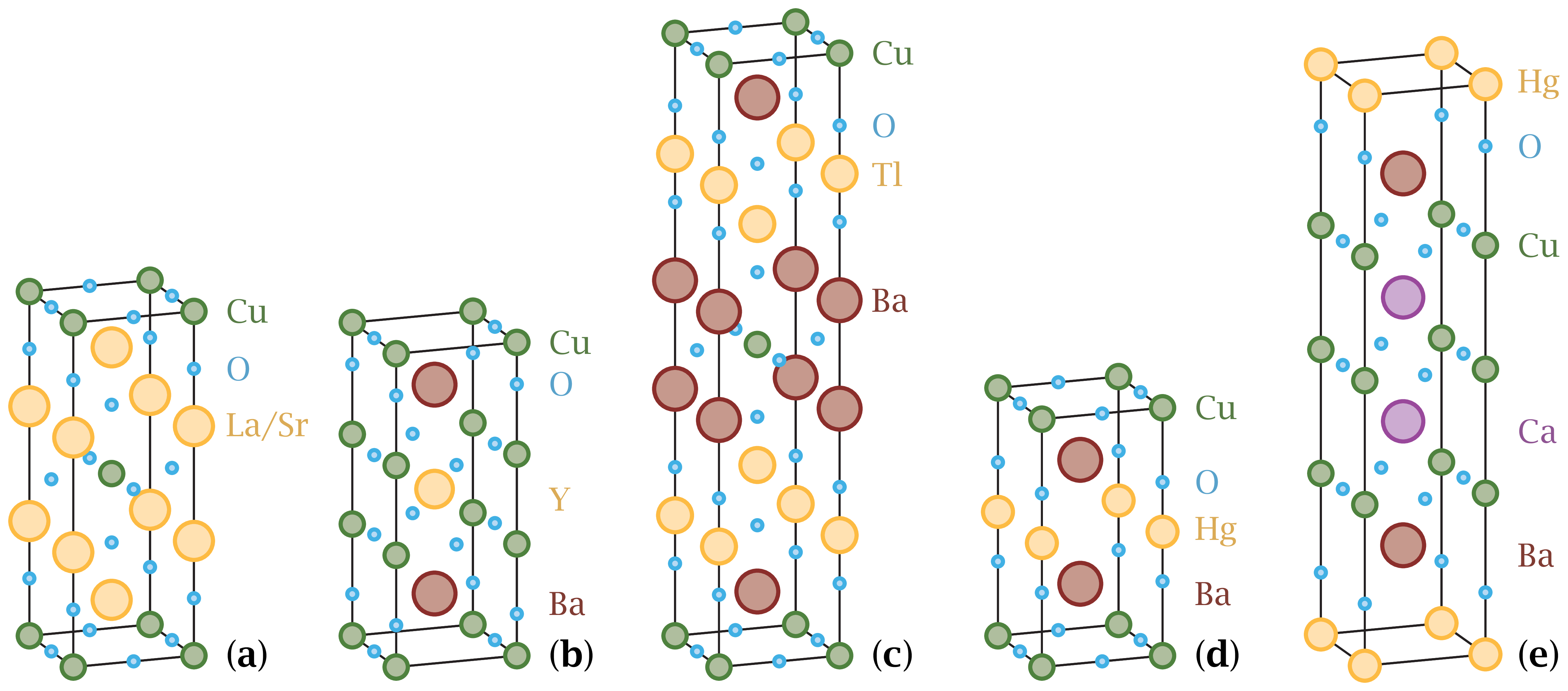
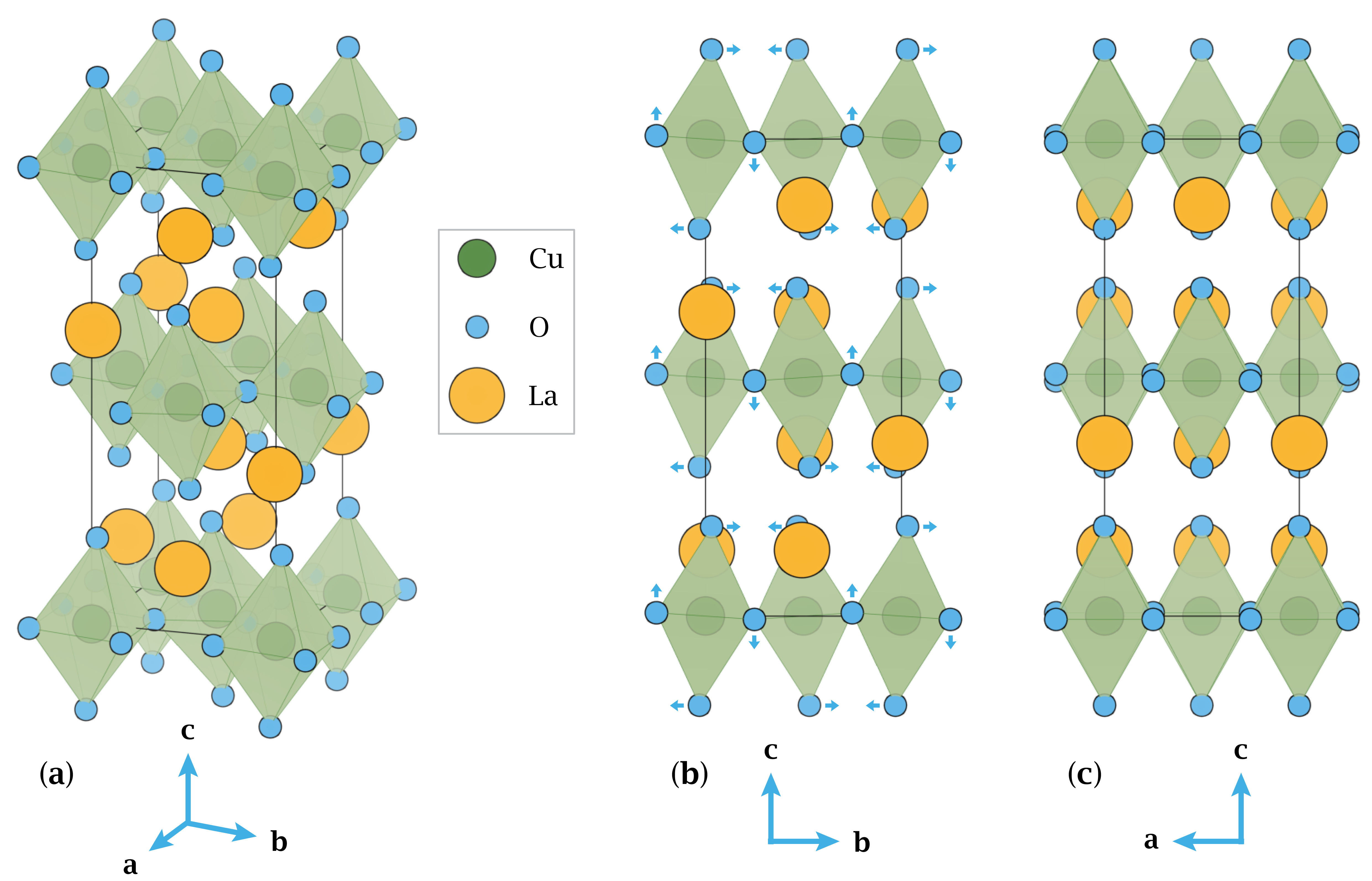
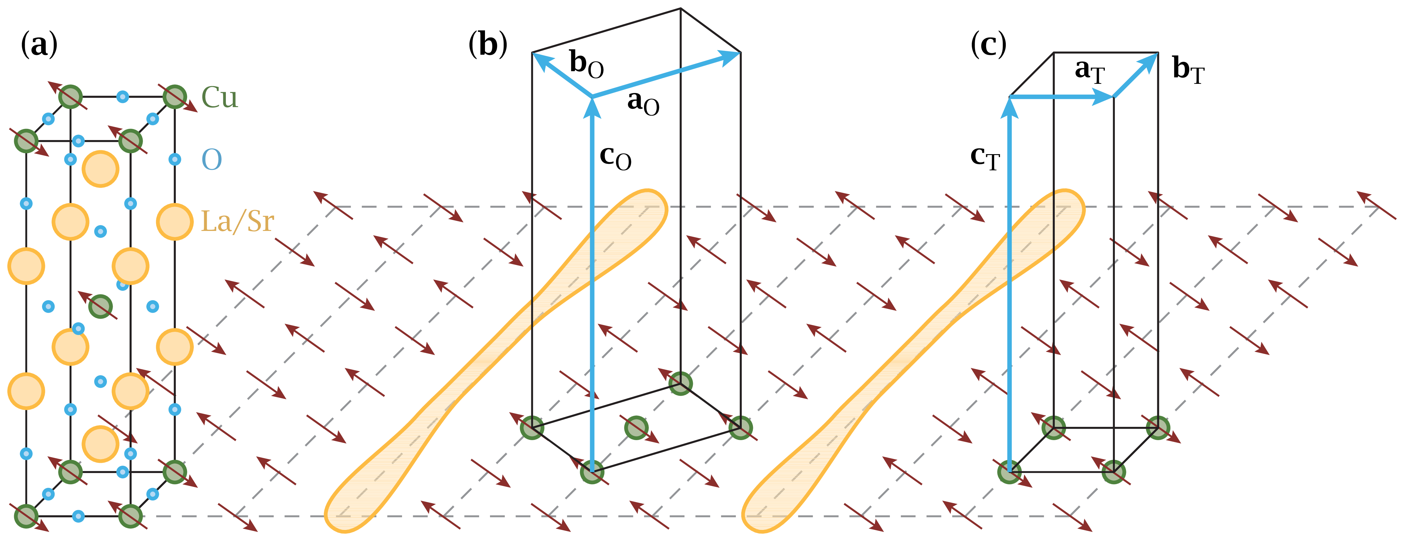
Figur 2.5: Examples of typical cuprate unit cells. Download links:PNG • αPNG • SVG • PDF. .
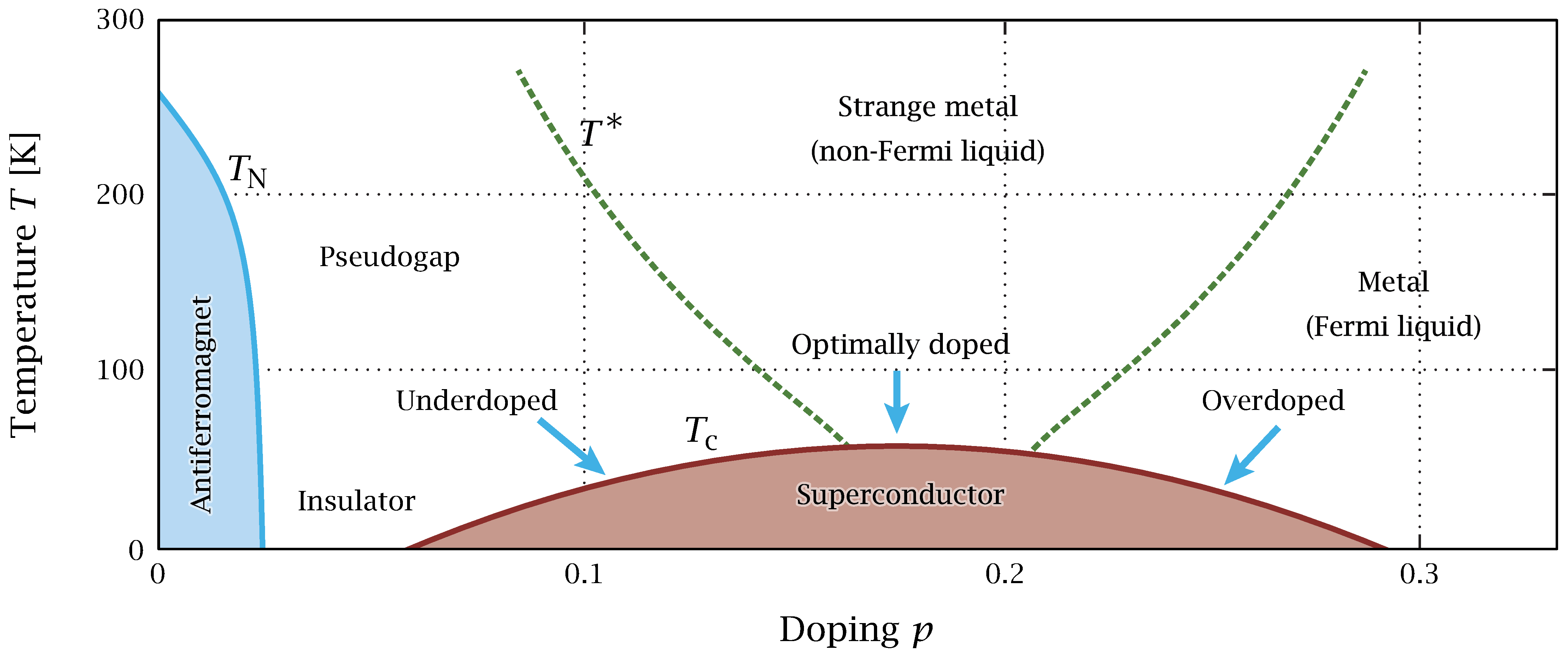
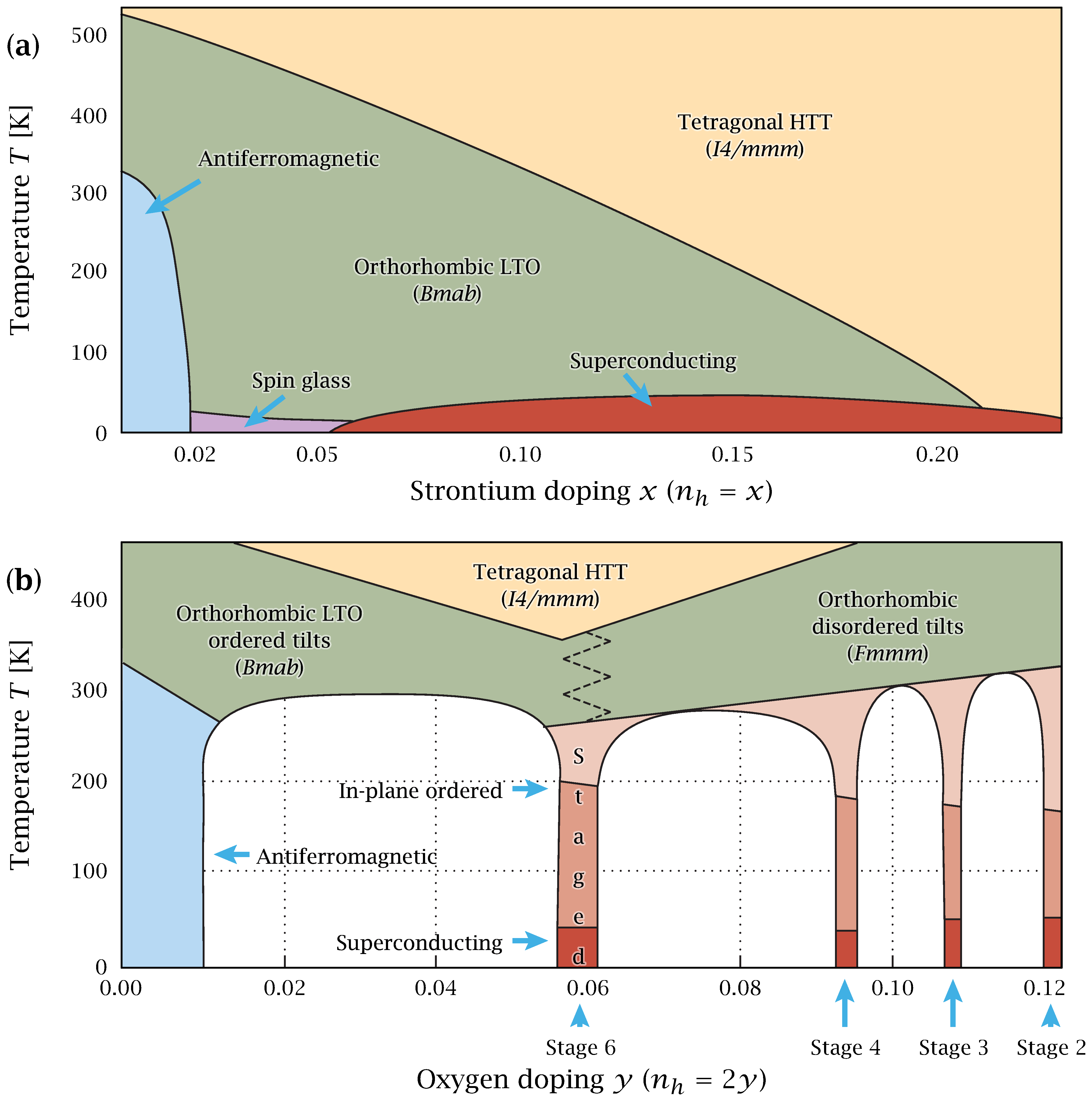
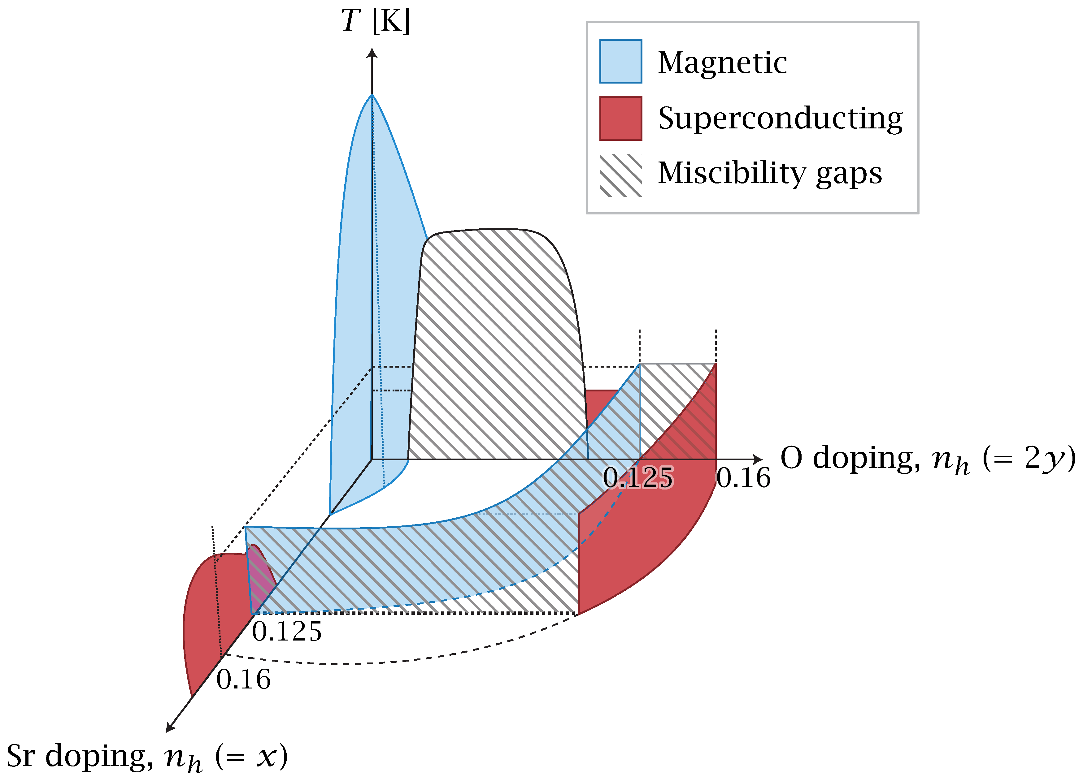
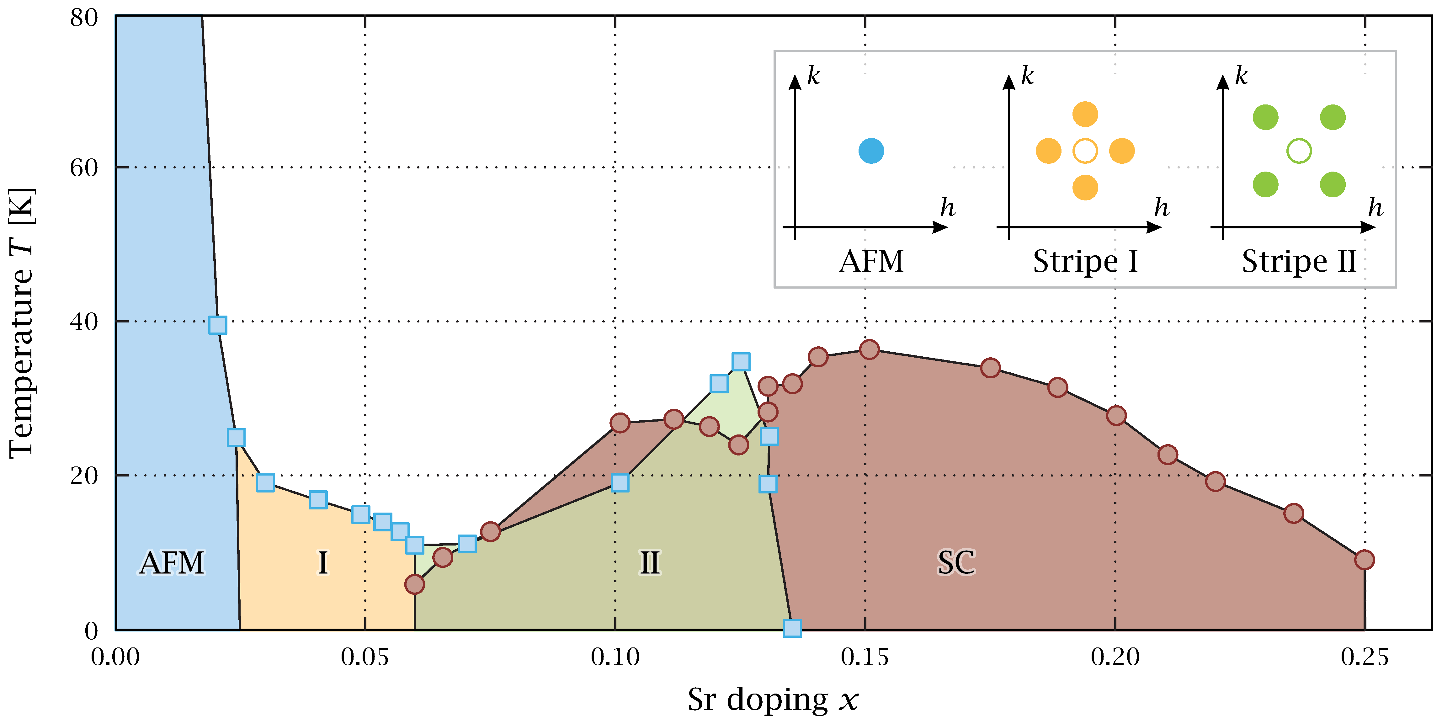
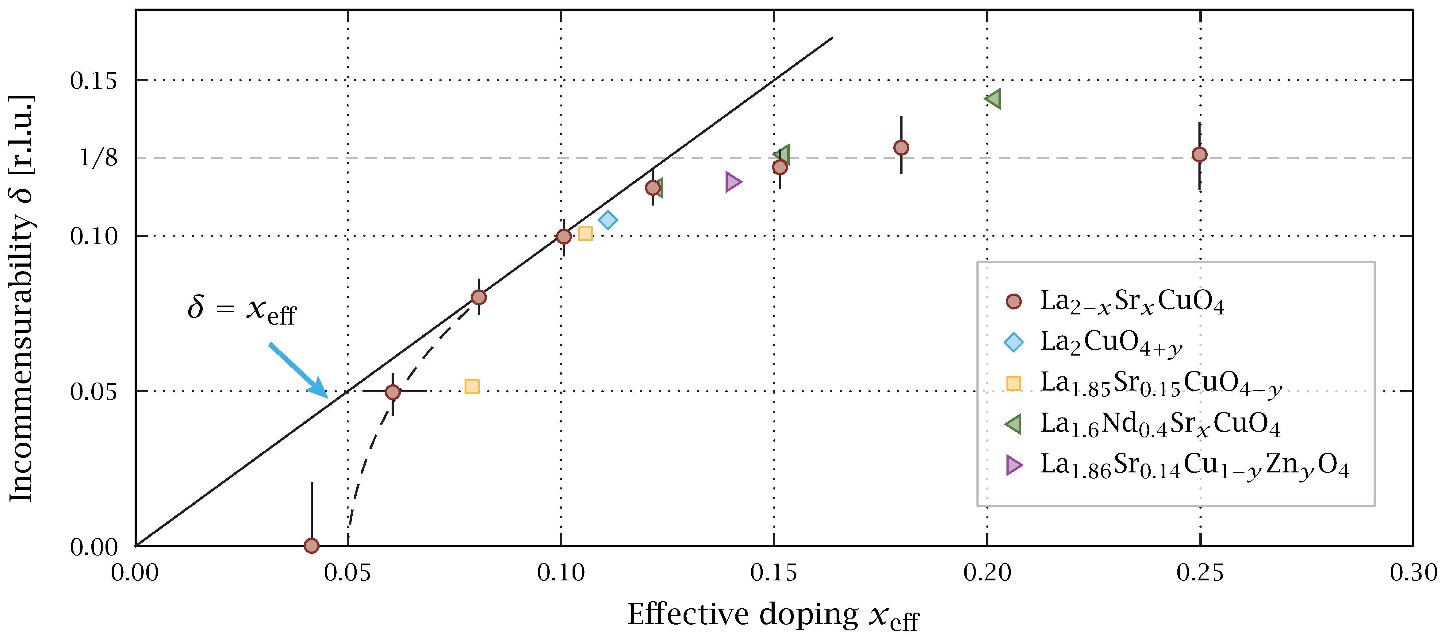
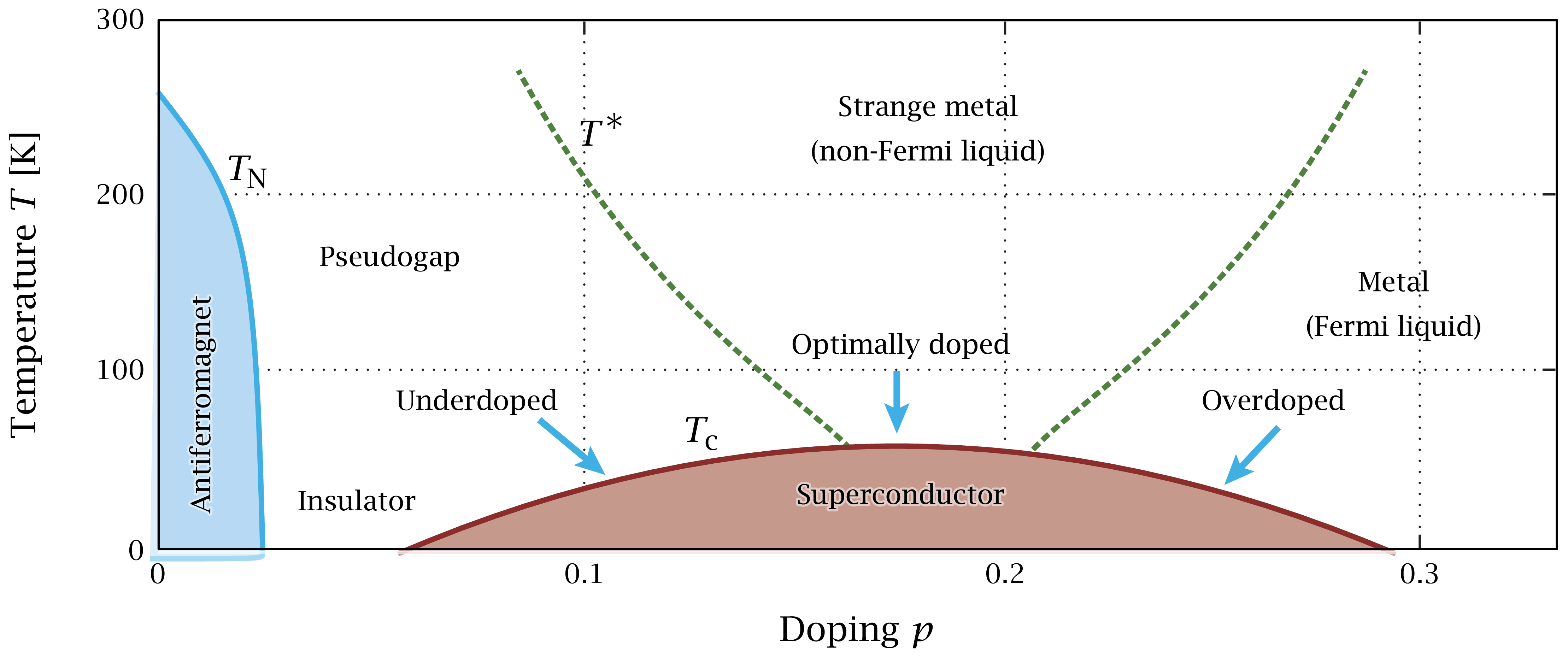
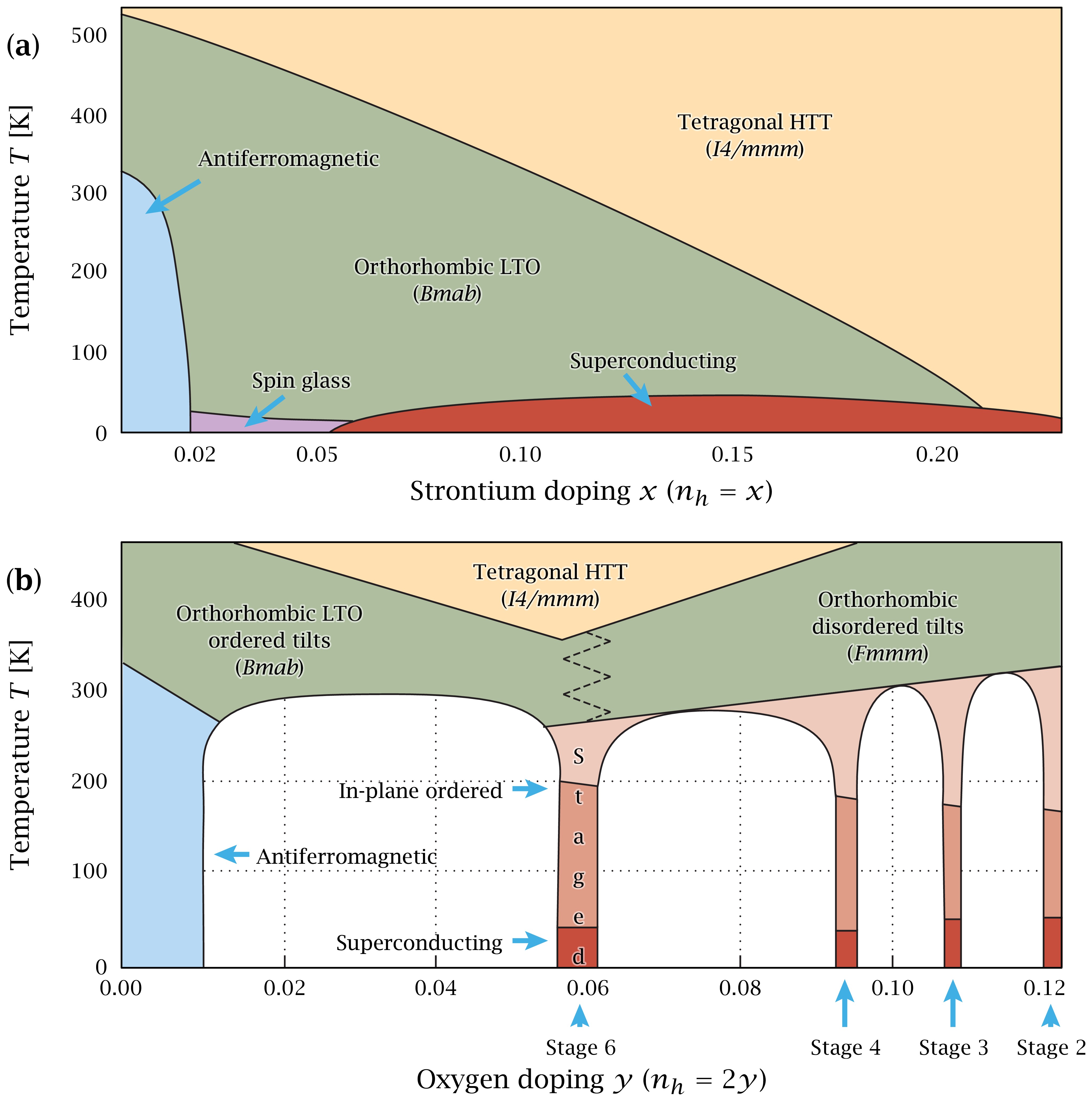
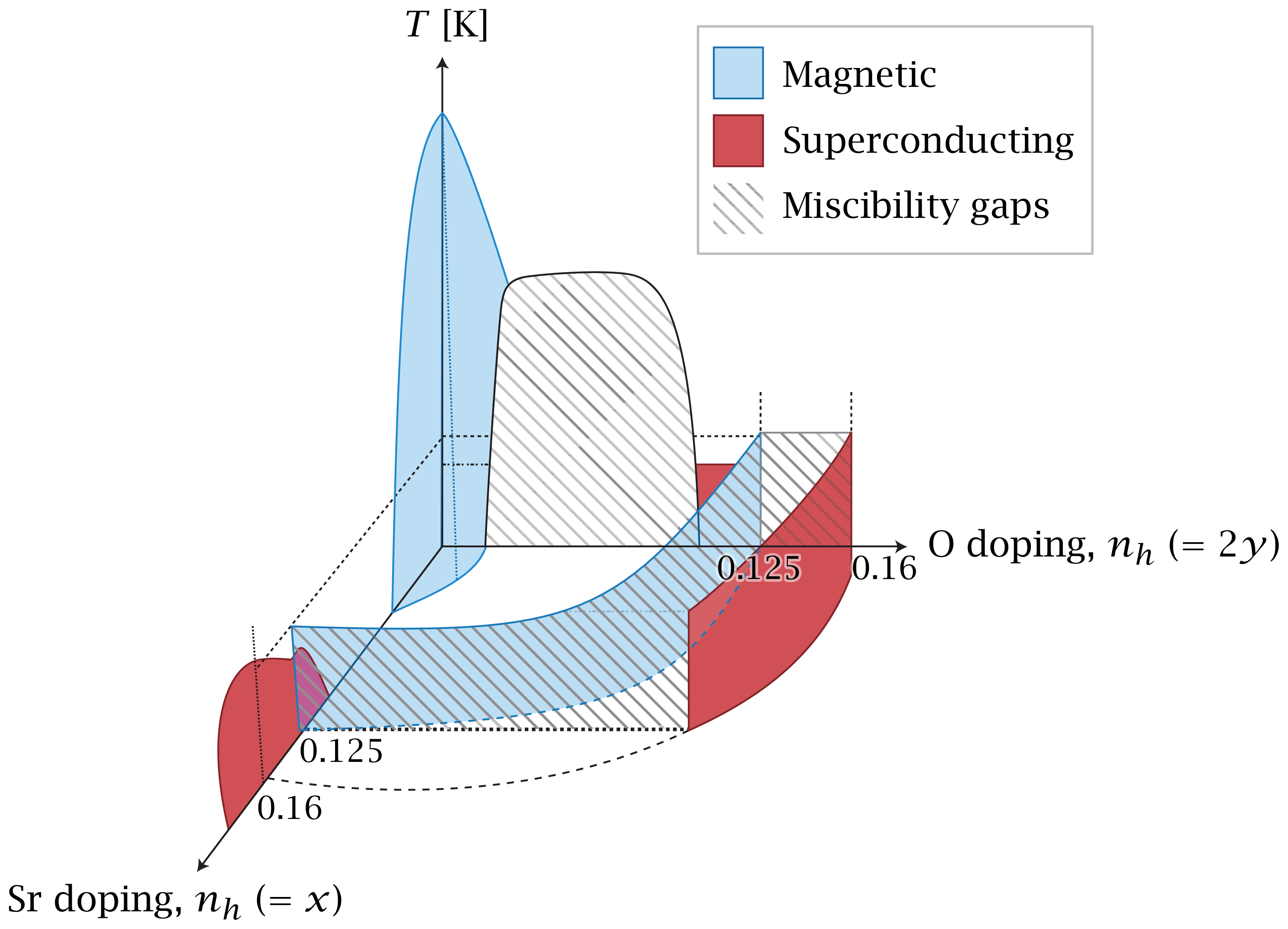
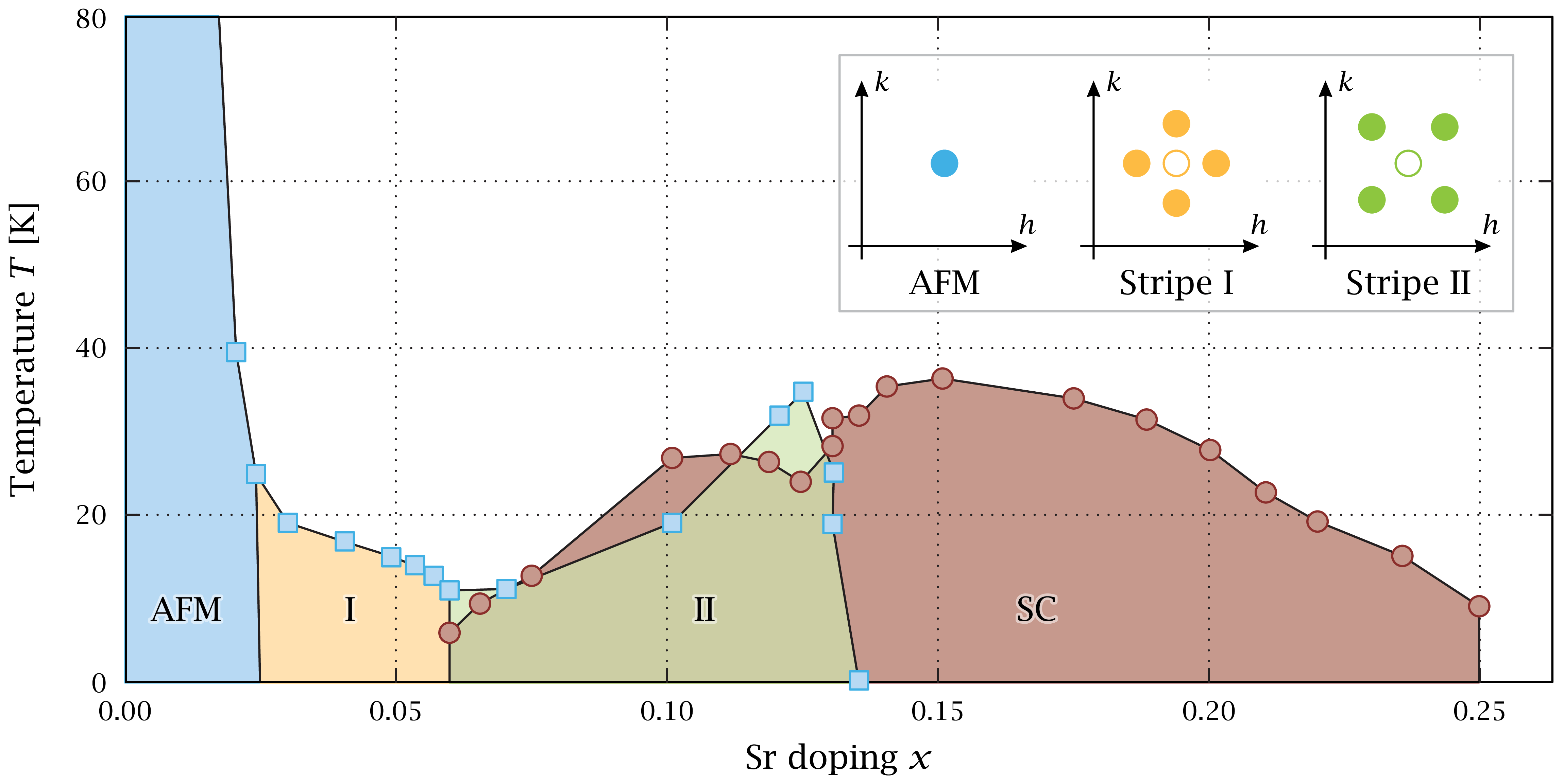
Figur 2.6: Typical phase diagram for a cuprate. Download links:PNG • αPNG • SVG • PDF. .
Krystallografi-illustrationer (kapitel 3)
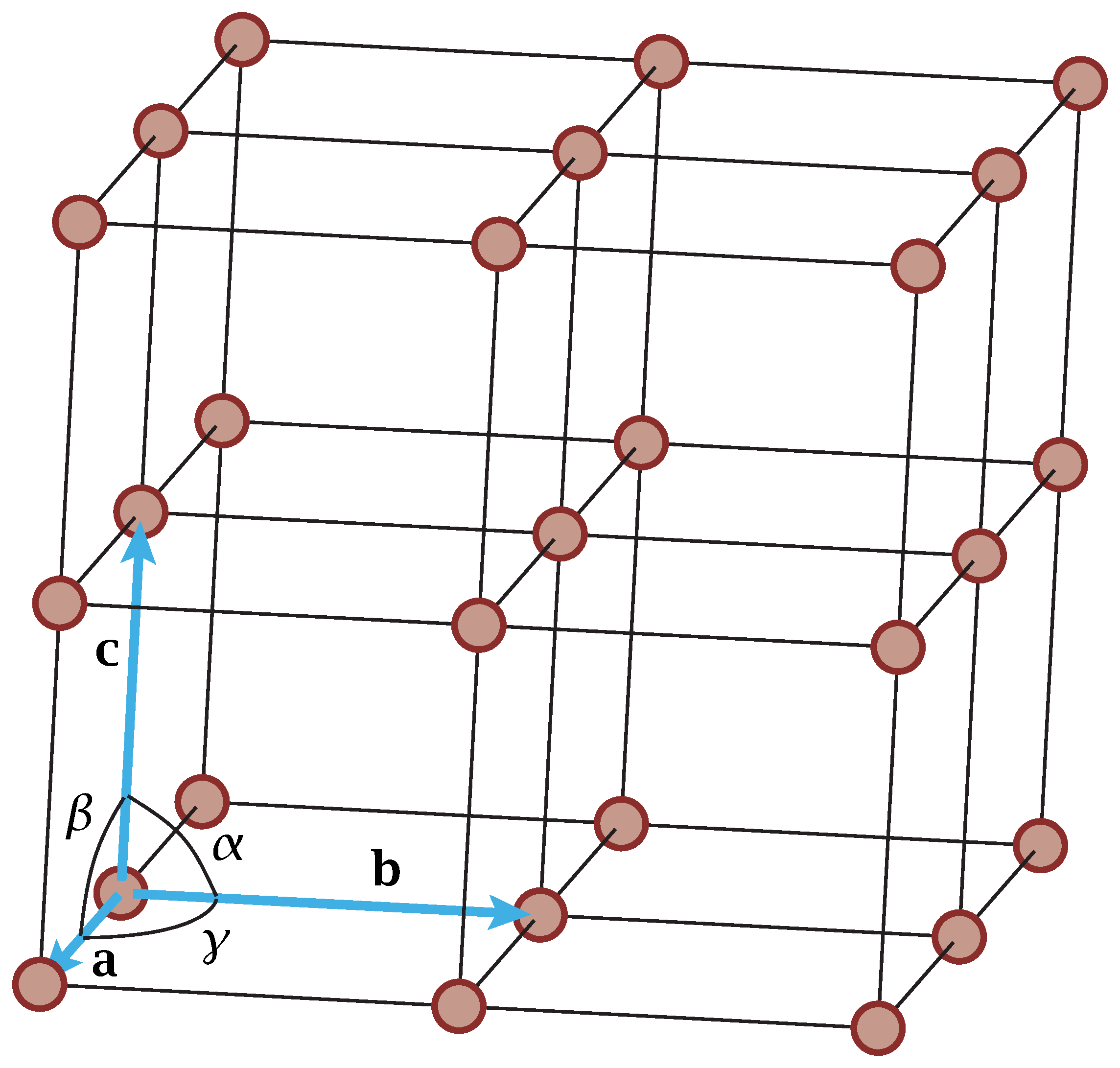
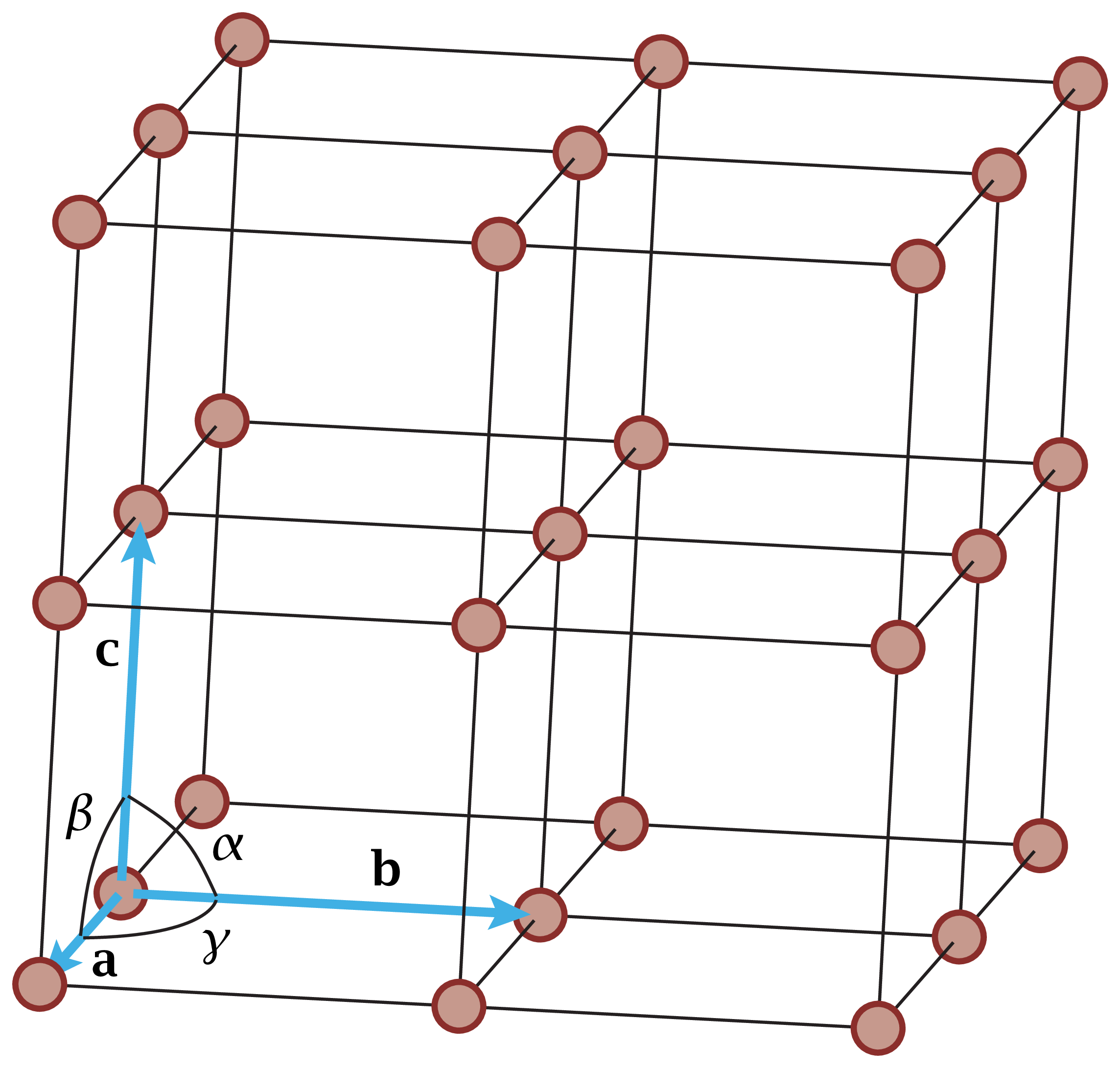
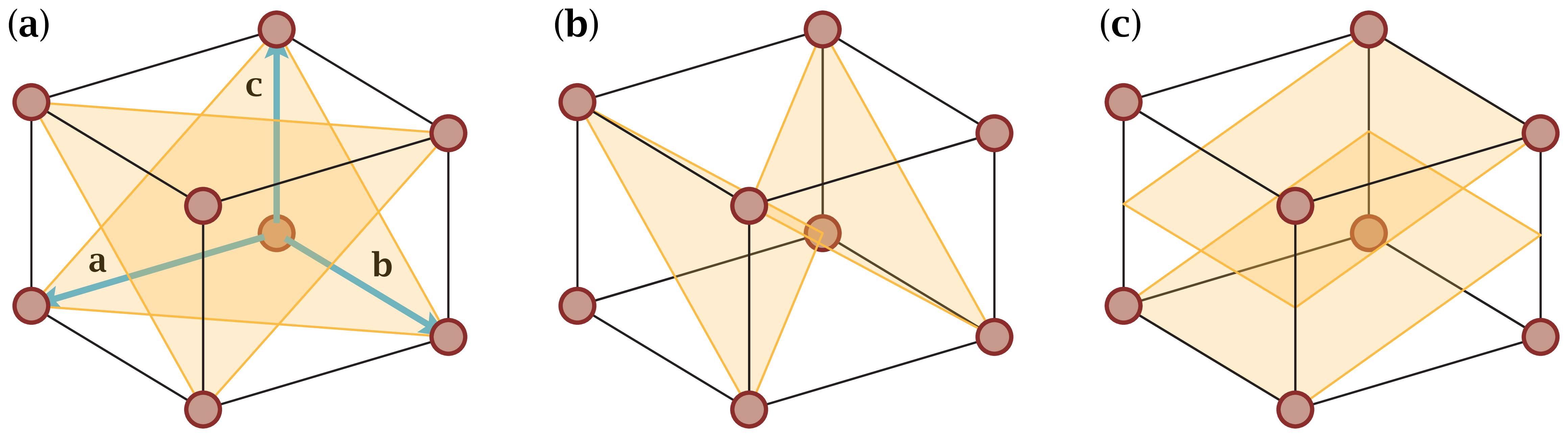
Figur 3.1: The lattice parameters in a standard crystal lattice. Download links:PNG • αPNG • SVG • PDF. .
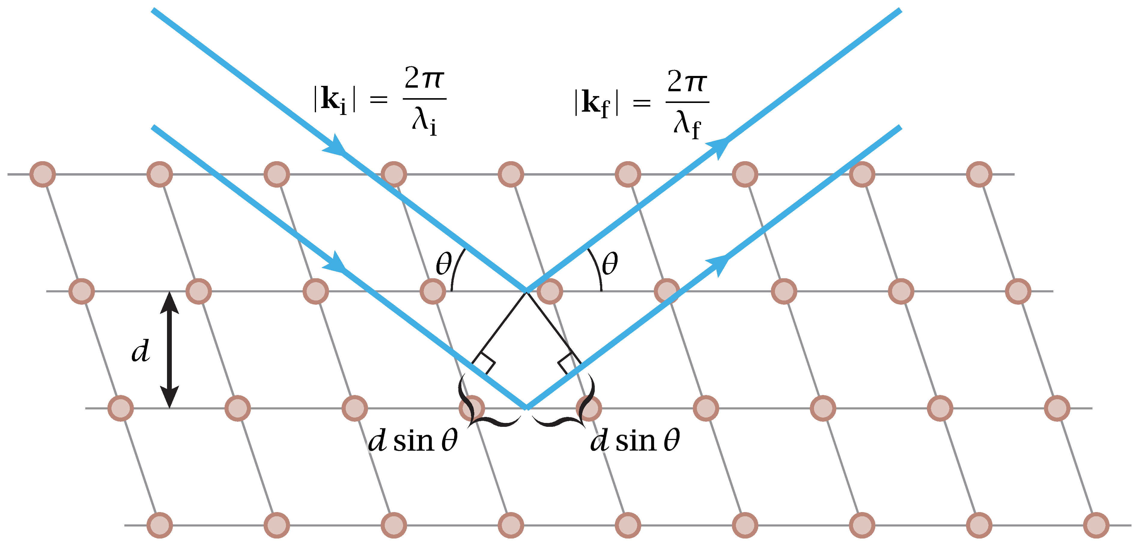
Figur 3.2: Simple examples of crystal planes in a standard crystal. Download links:PNG • αPNG • SVG • PDF. .
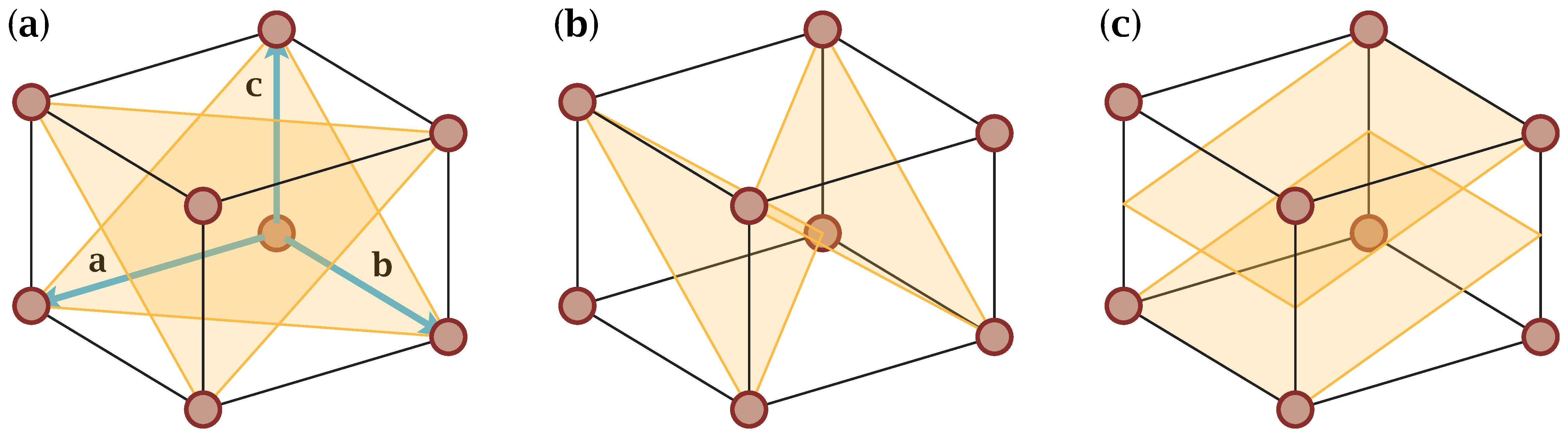
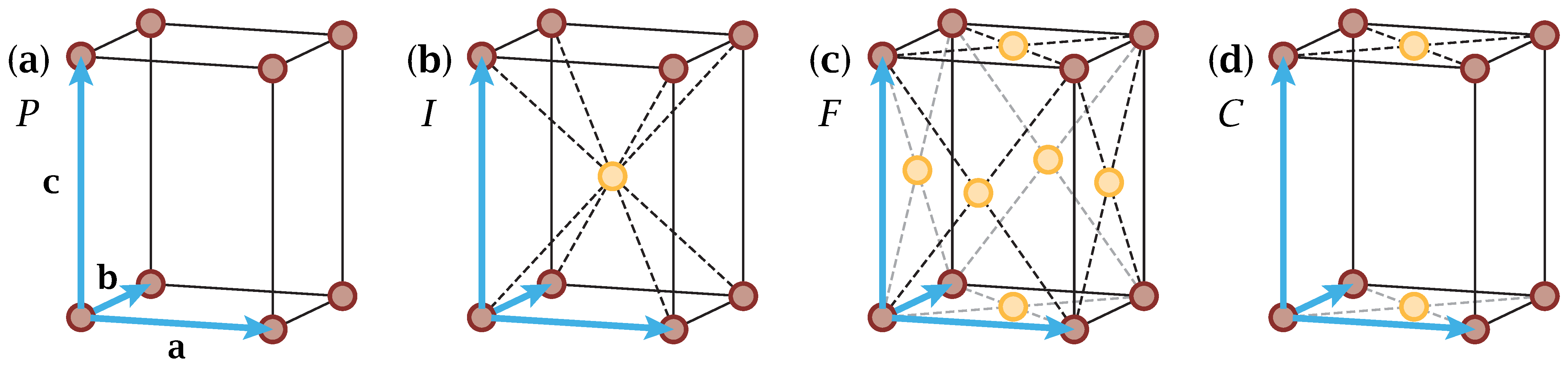
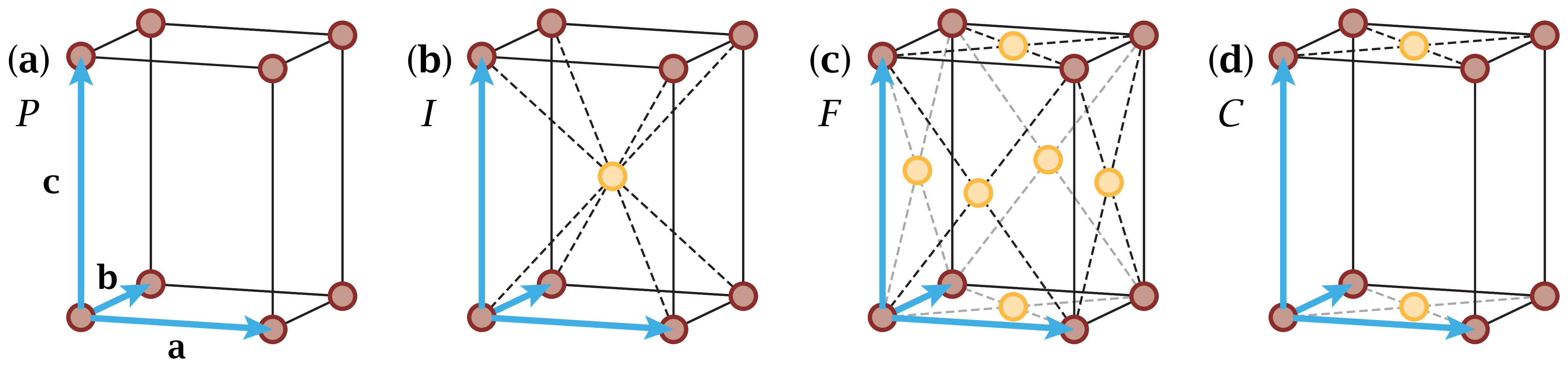
Figur 3.3: The P, I, F, and C lattice centrings. Download links:PNG • αPNG • SVG • PDF. .
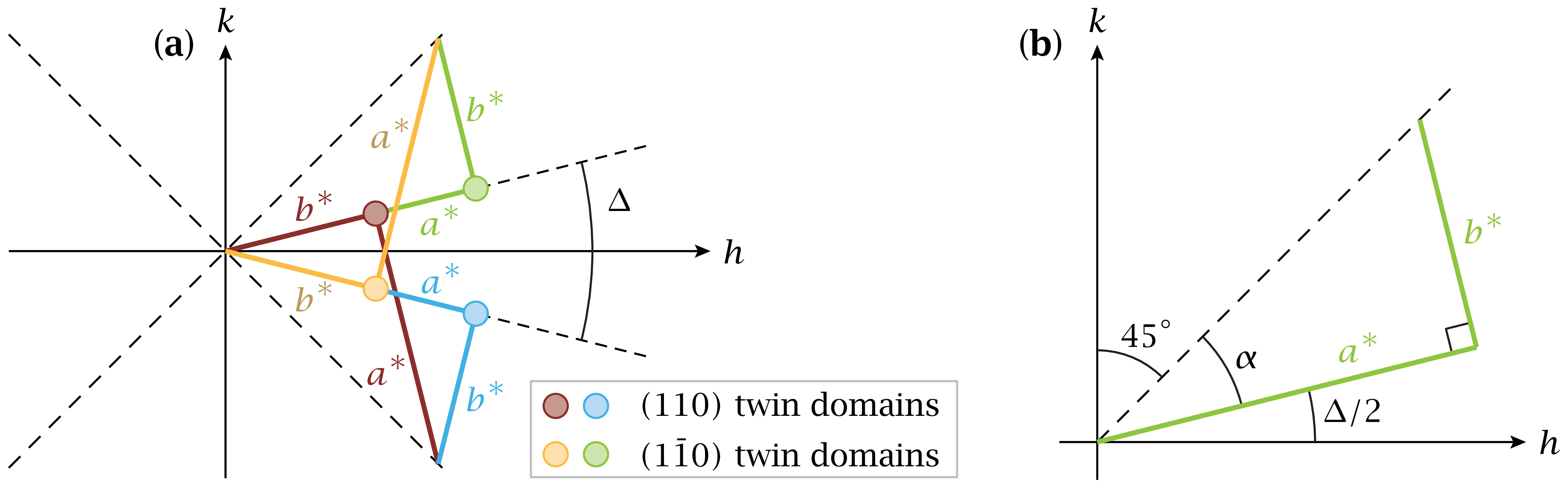
Figur 6.1: Example of attempted detwinning. Download links:PNG • SVG • PDF. .
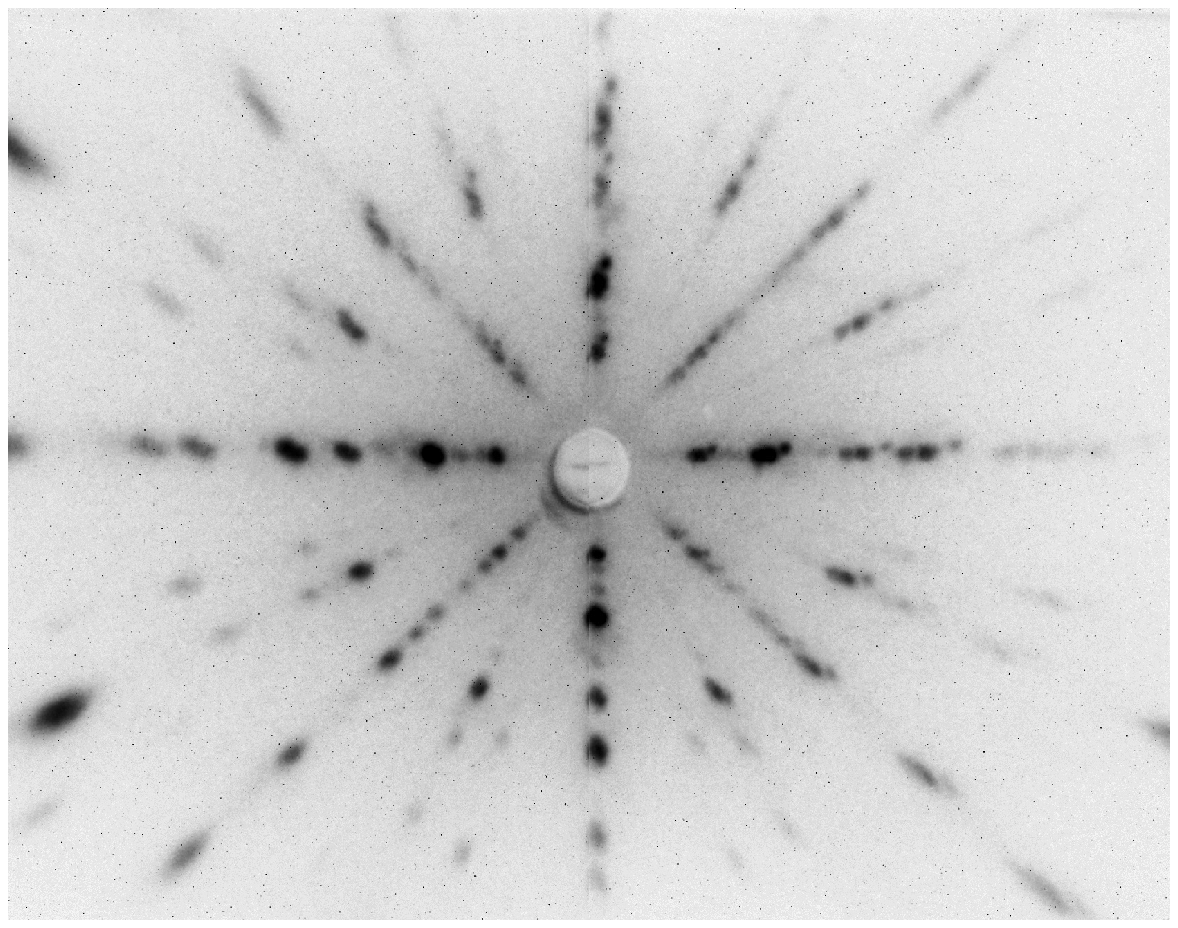
Figur 6.2: Example of neutron-Laue image of a La(2)CuO(4+y) sample. Download links:PNG • SVG • PDF. .
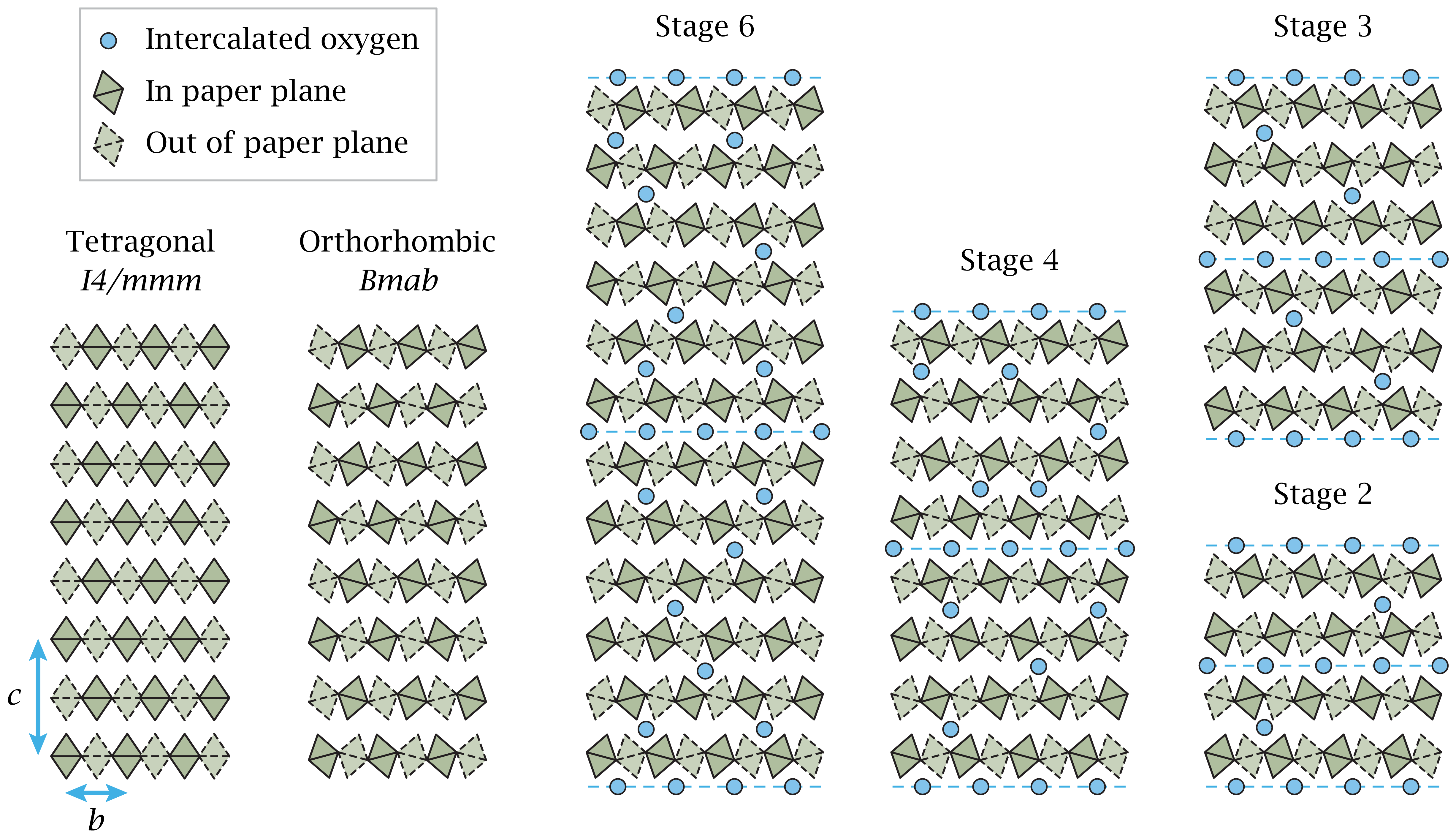
Staging-illustrationer (kapitel 7)
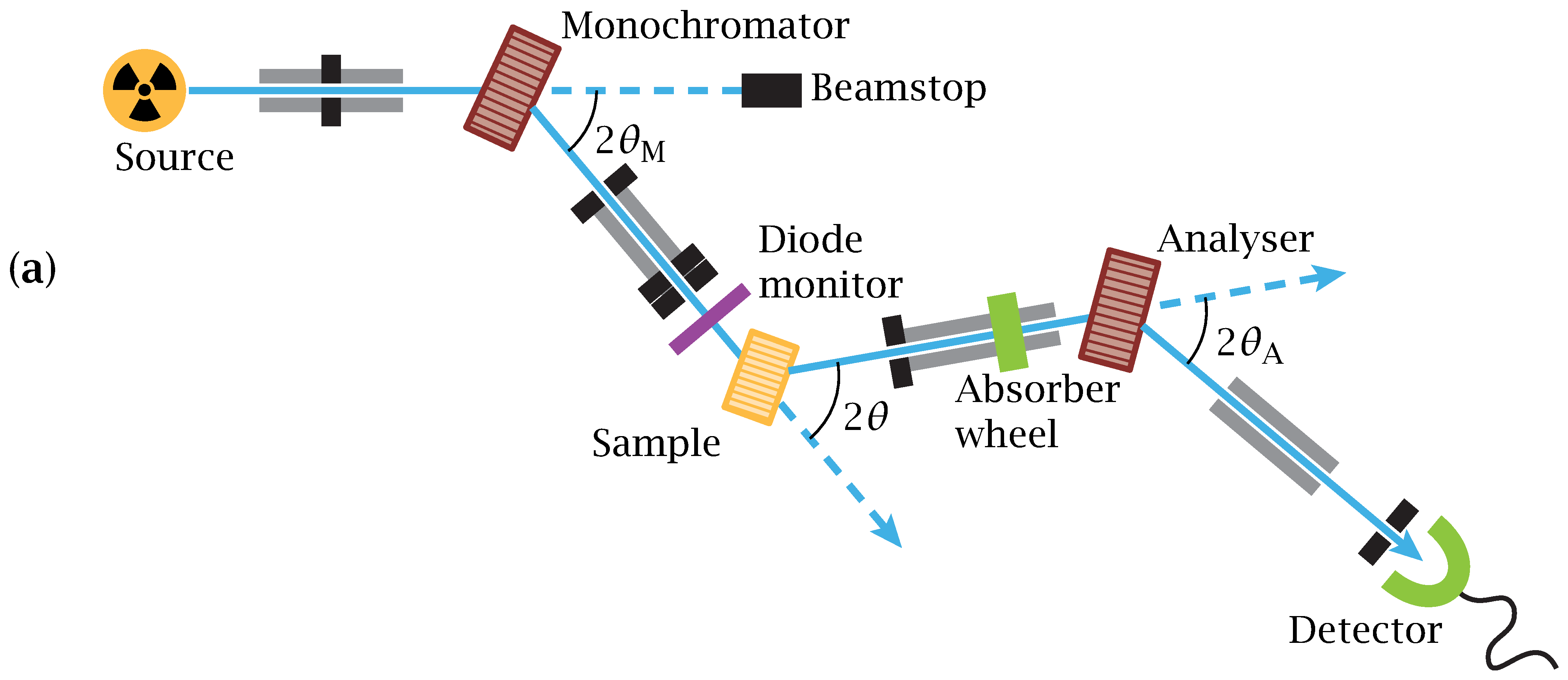
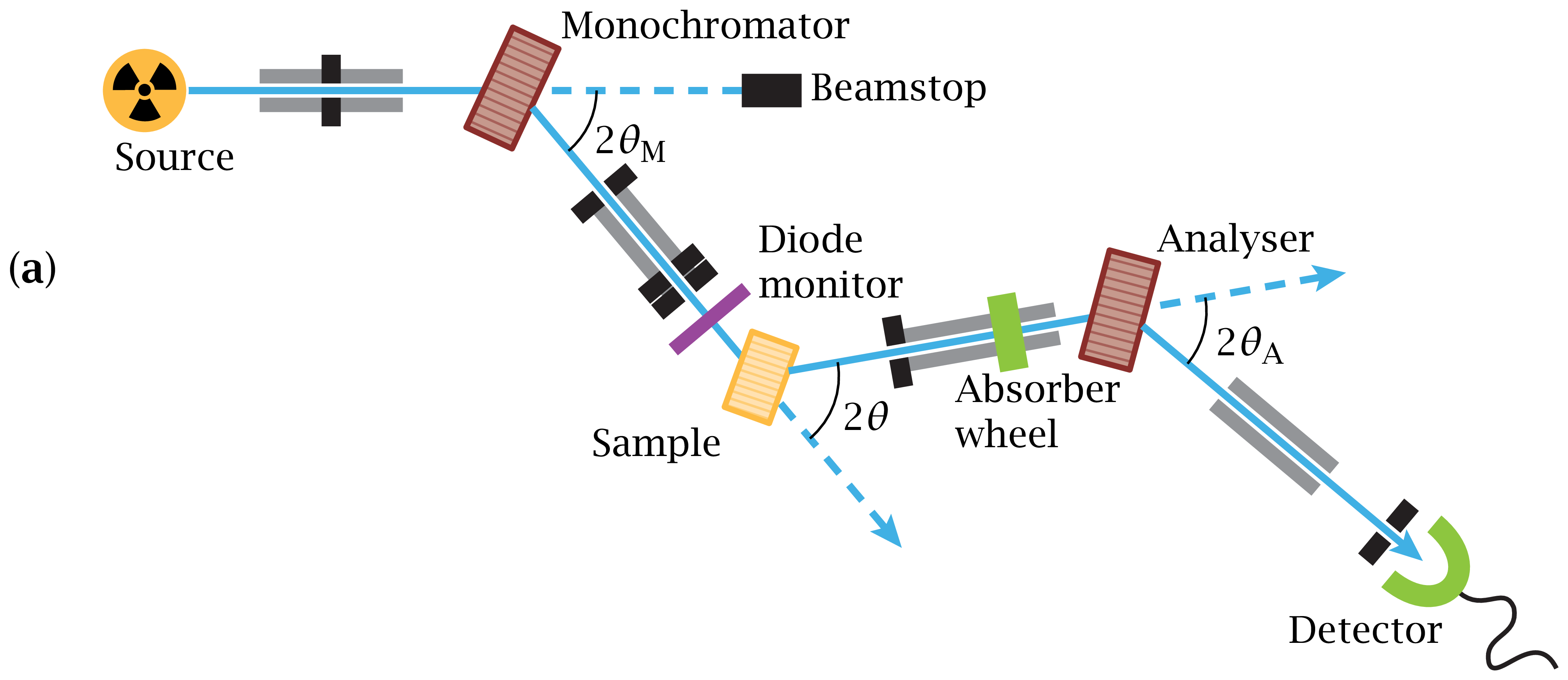
Figur 7.1(a): Overview sketch of the BW5 instrument. Download links:PNG • αPNG • SVG • PDF. .
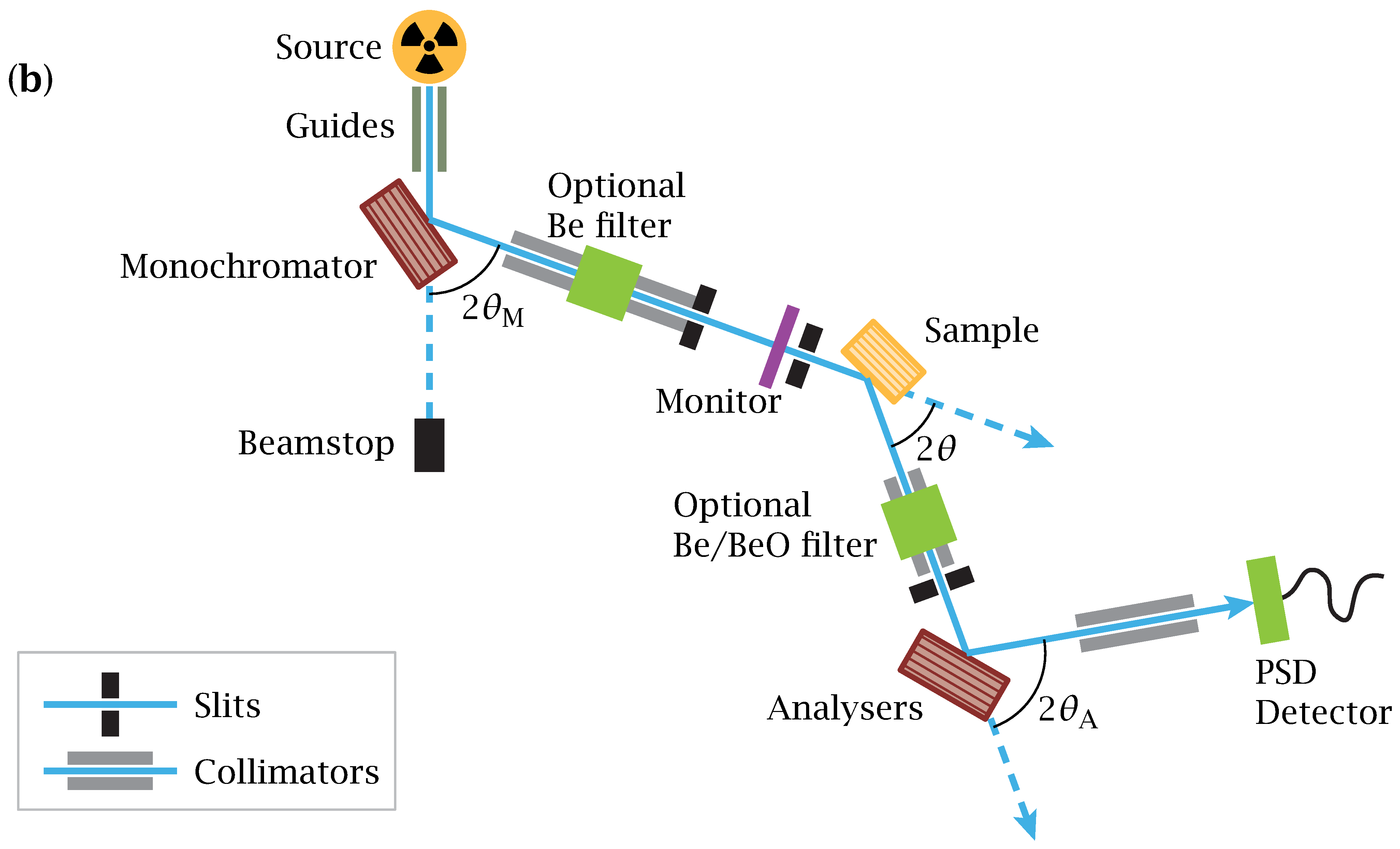
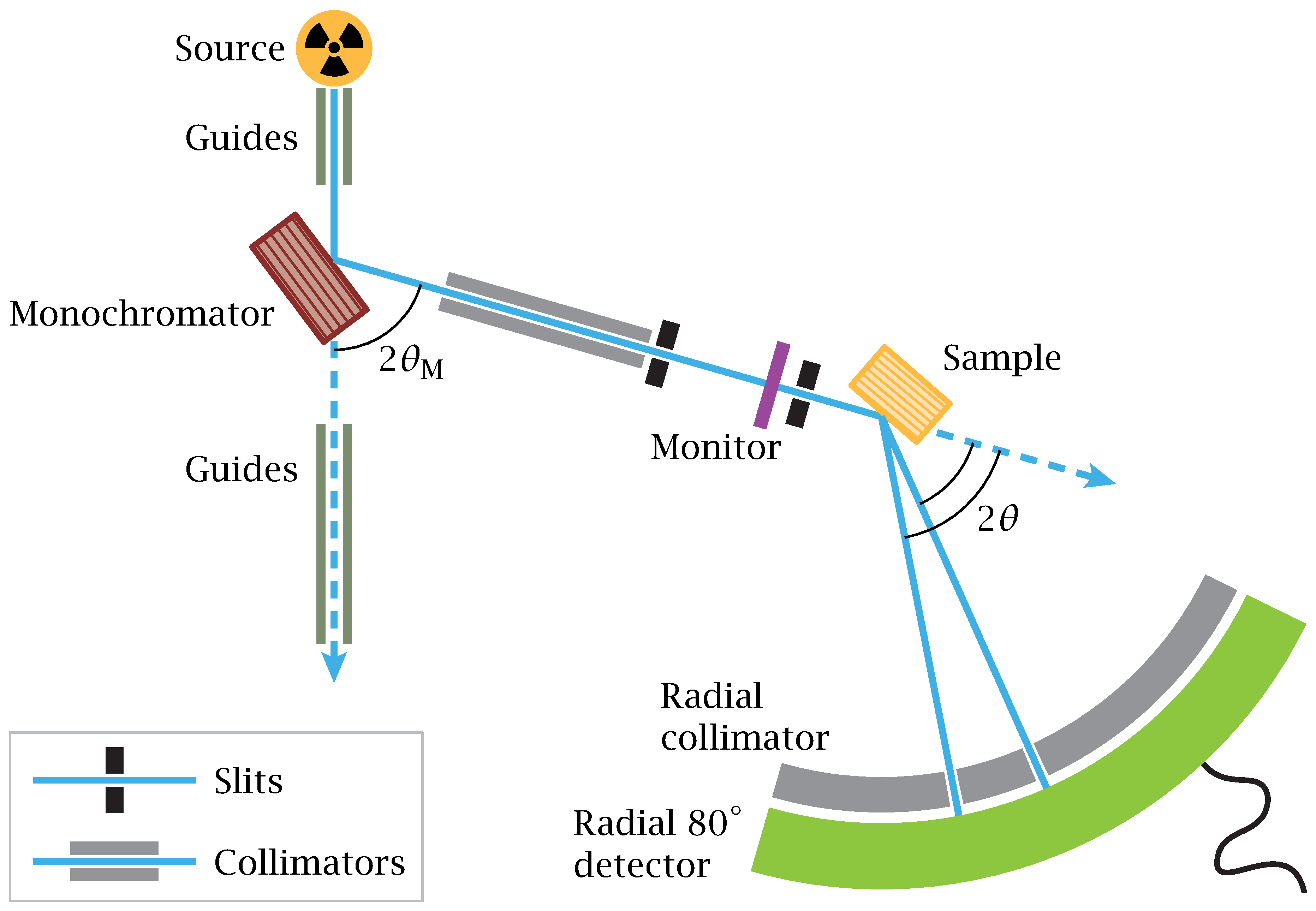
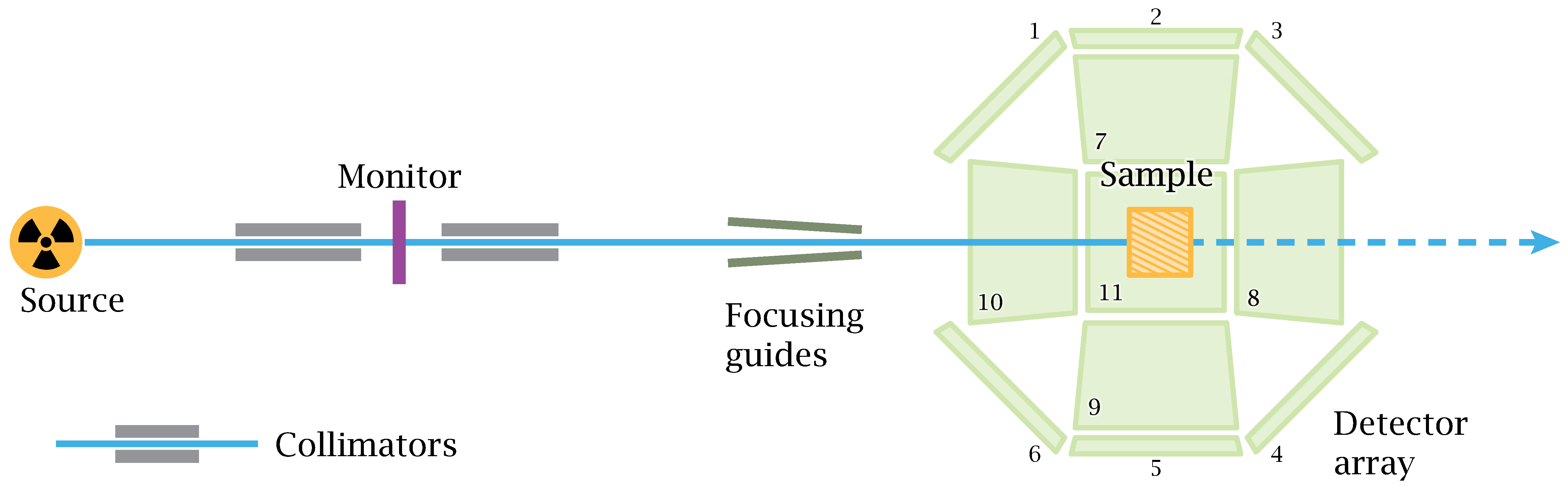
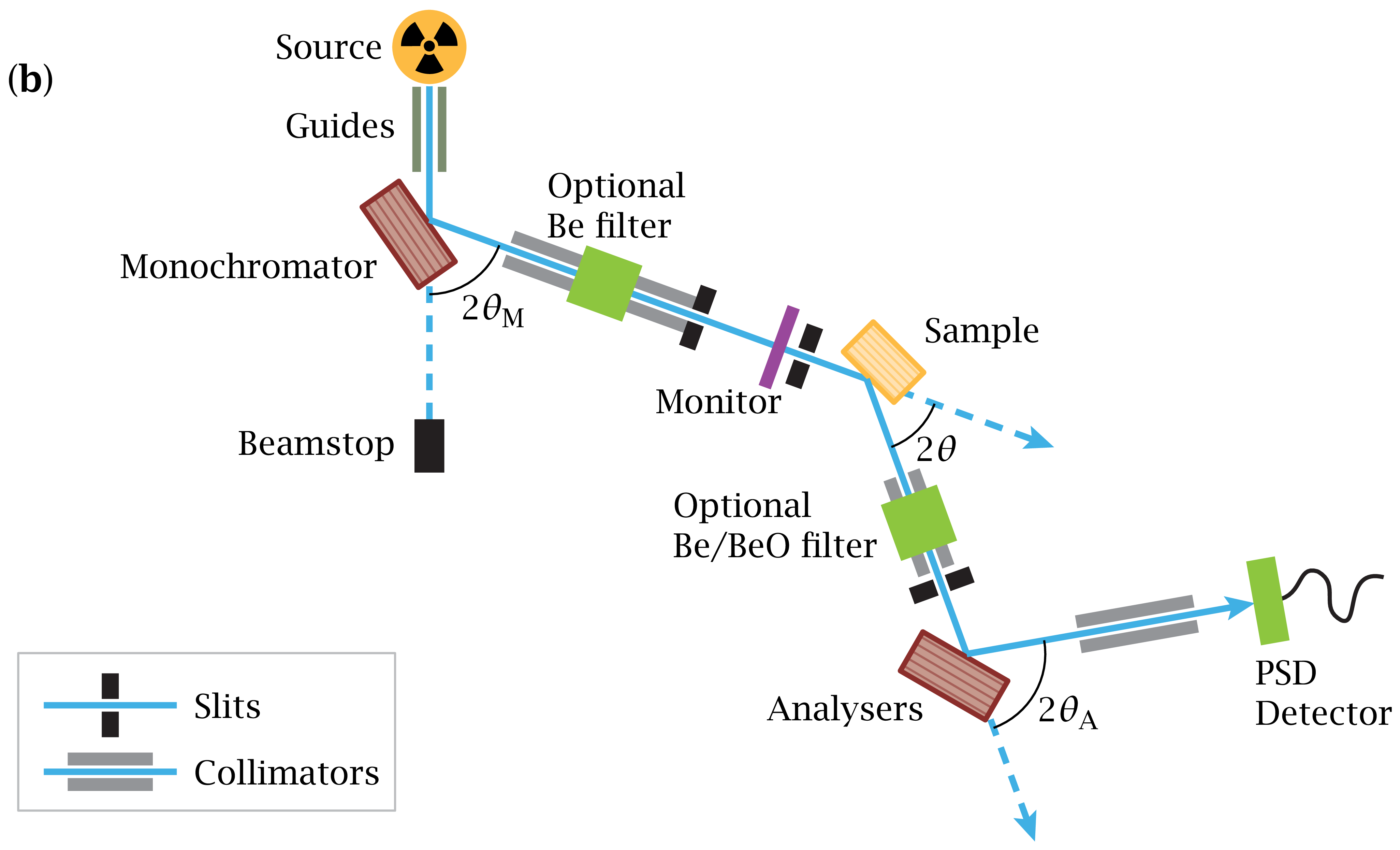
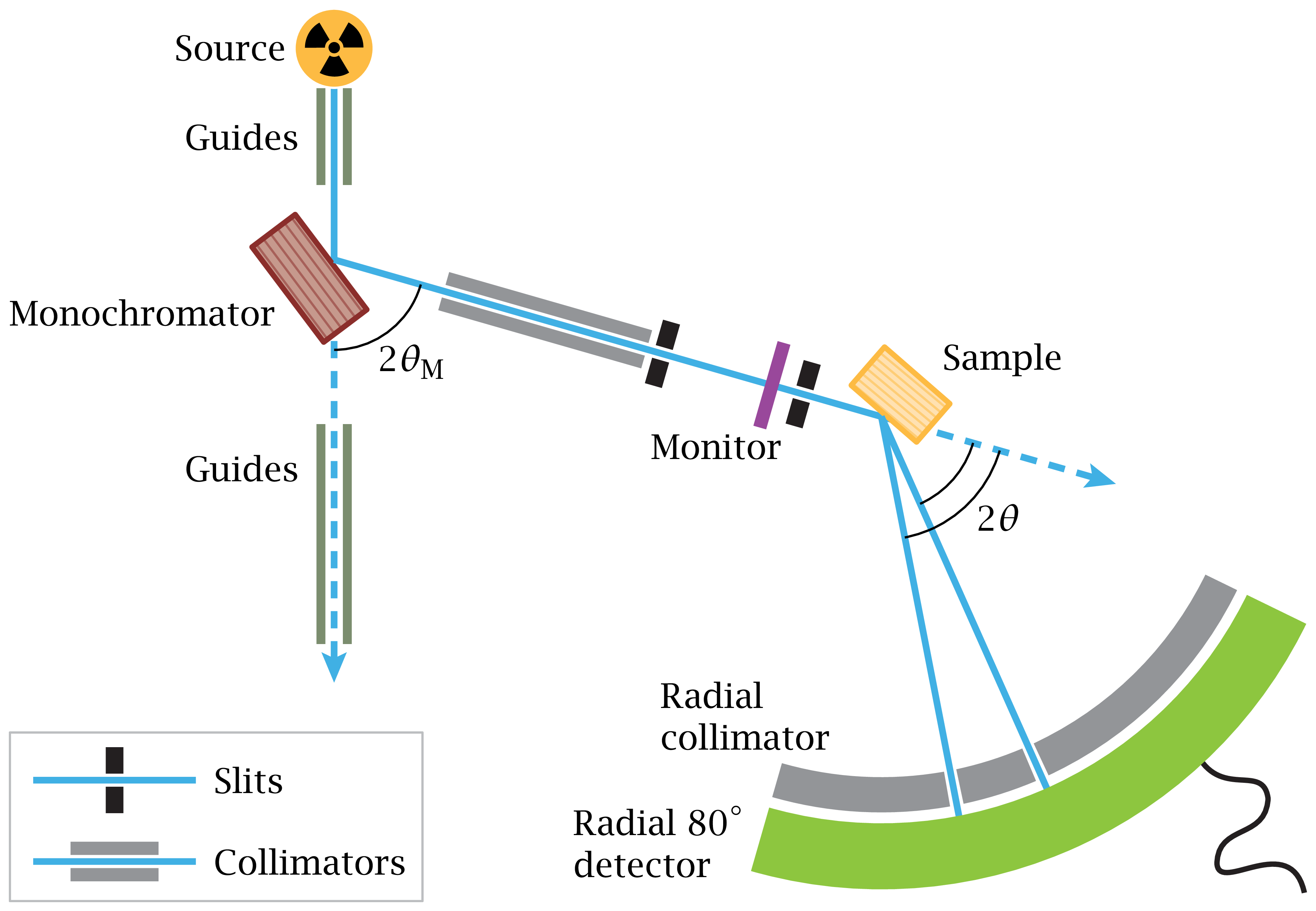
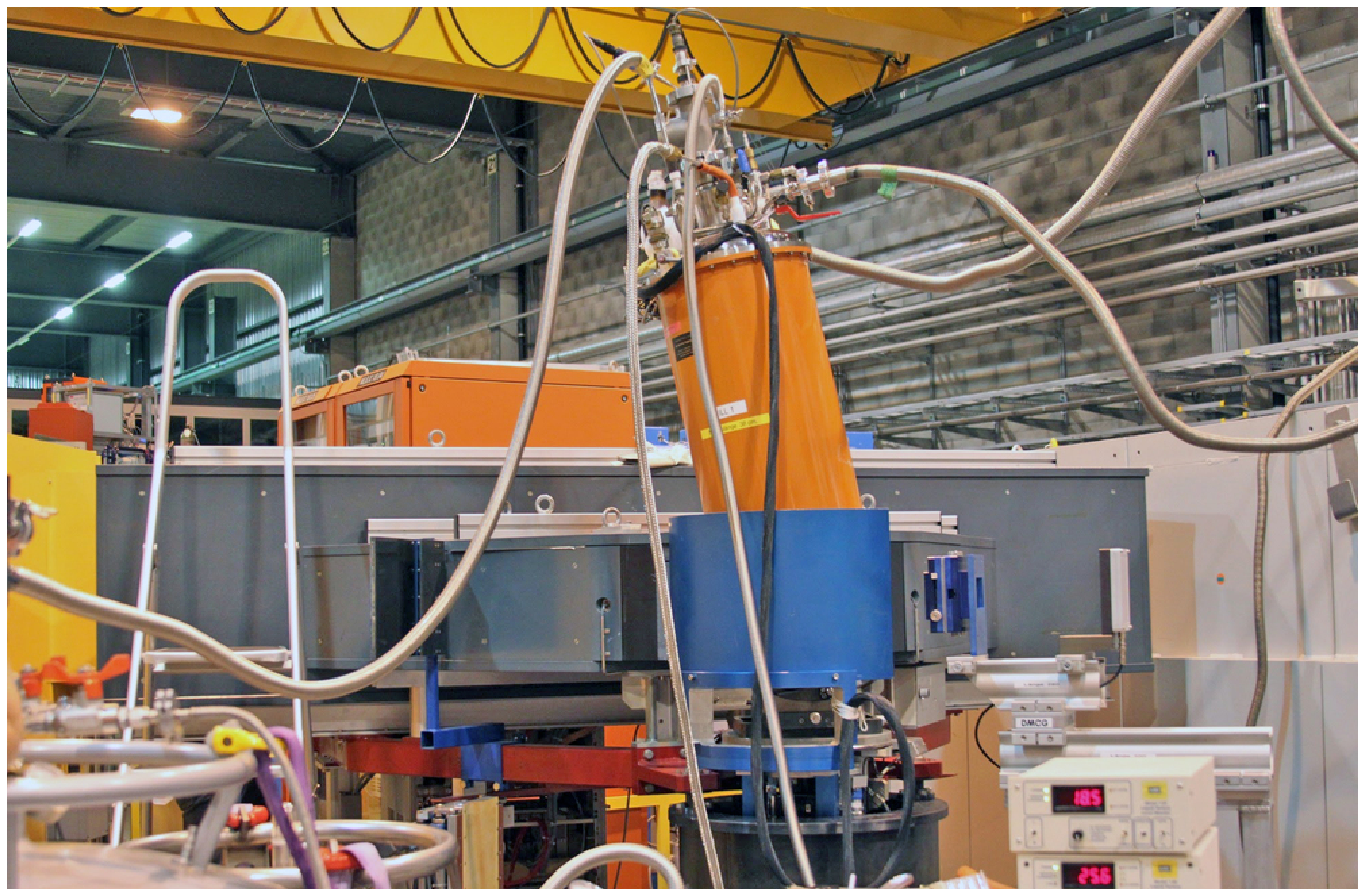
Figur 7.1(b): Overview sketch of the RITA-II instrument. Download links:PNG • αPNG • SVG • PDF. .
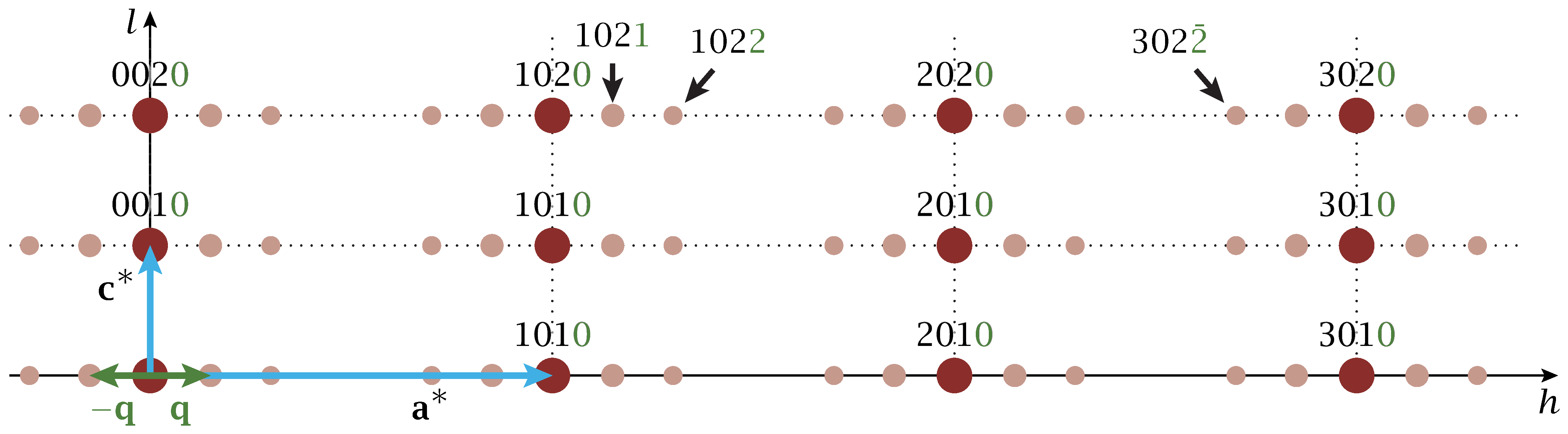
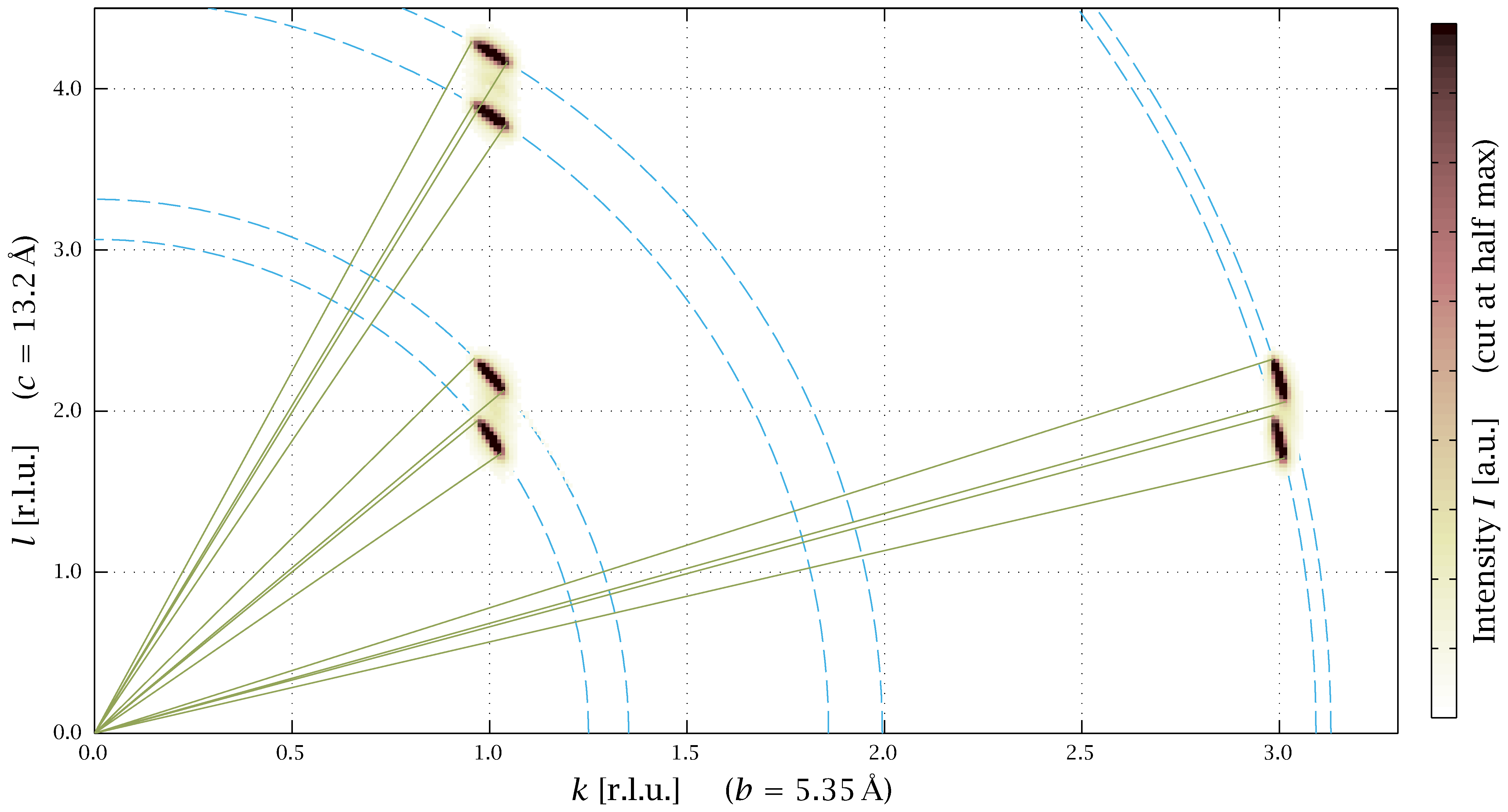
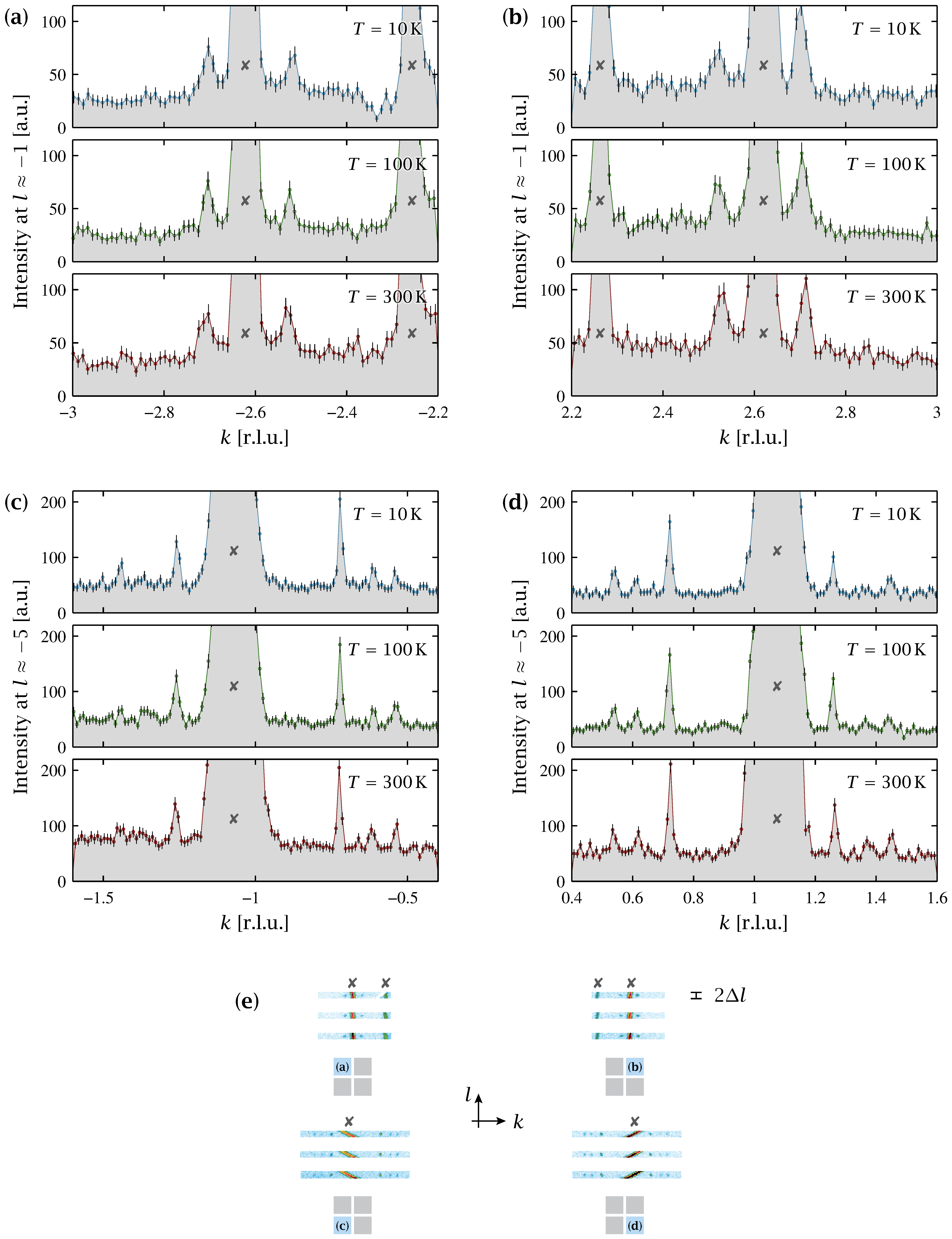
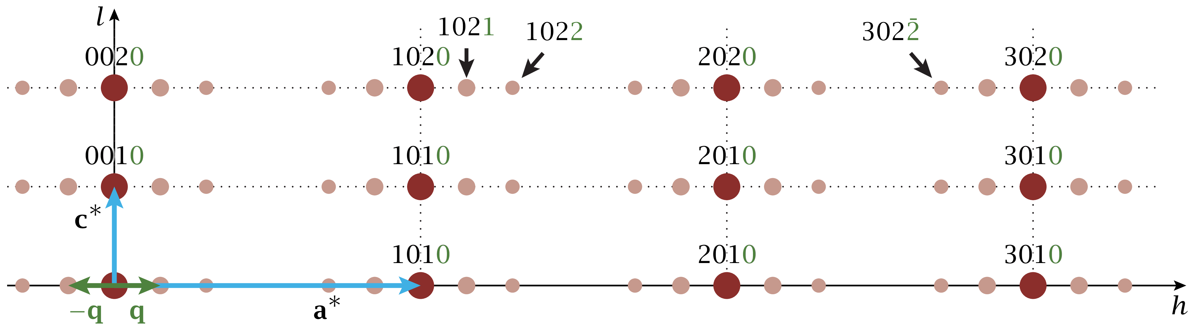
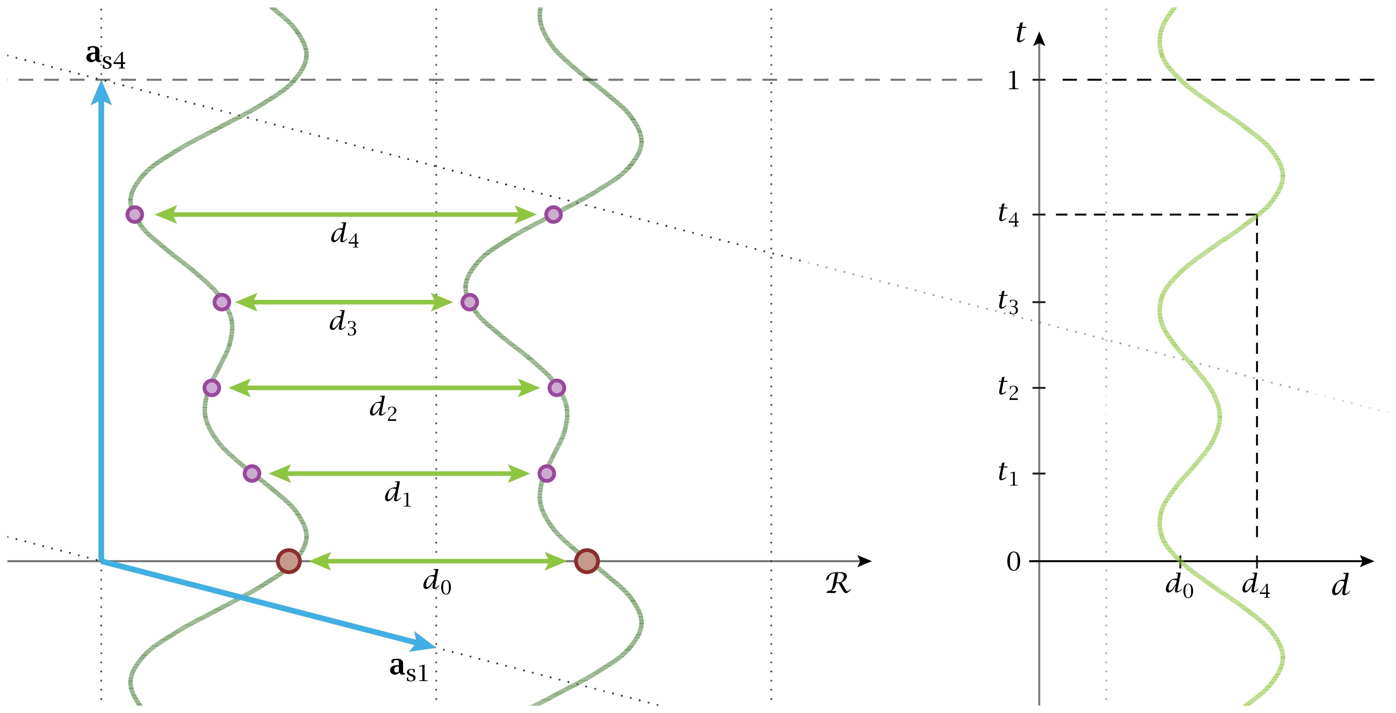
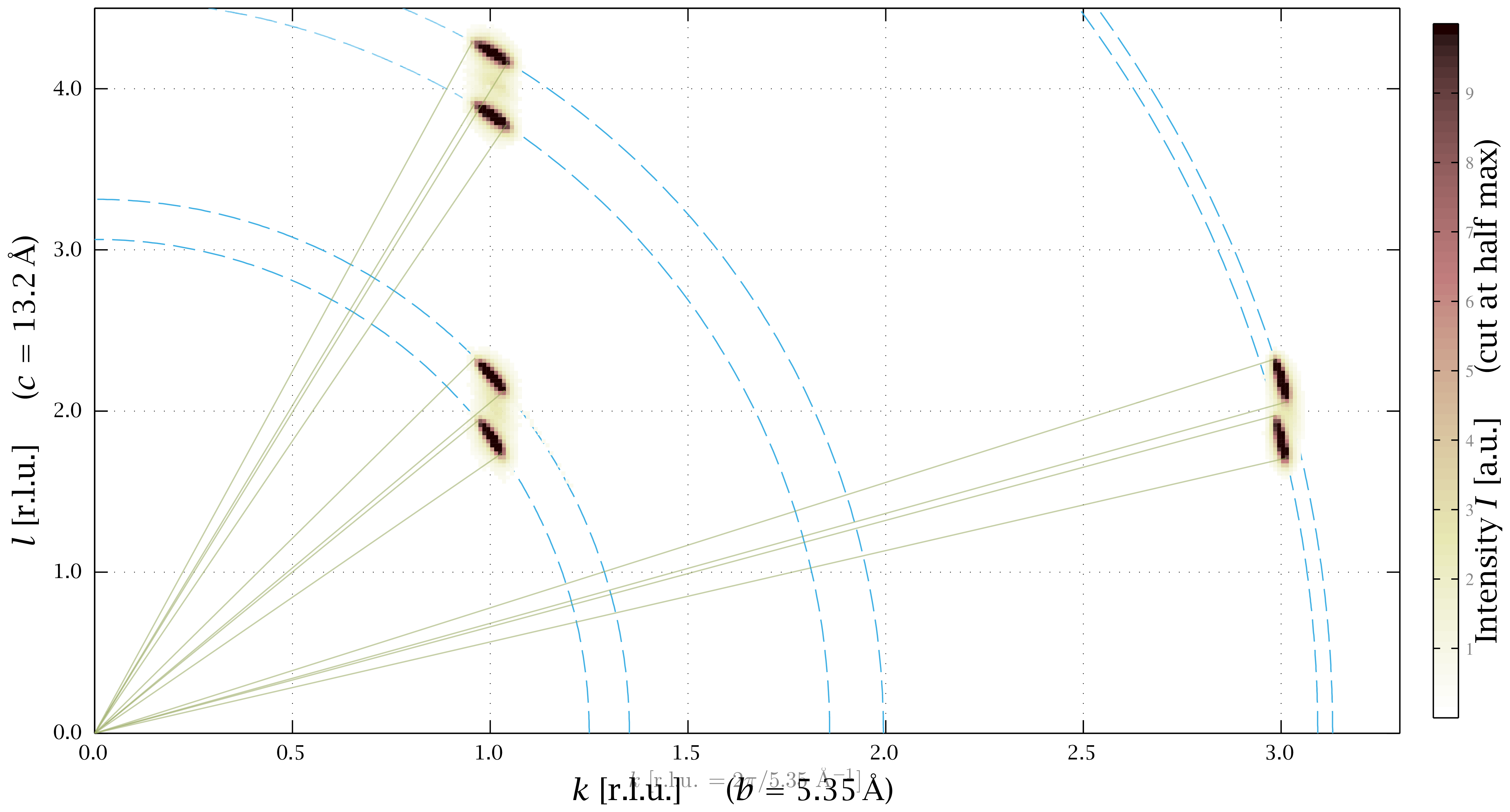
Figur 7.2: Reciprocal-space plane showing Bmab reflections splitting along l due to staging. Download links:PNG • αPNG • SVG • PDF. .
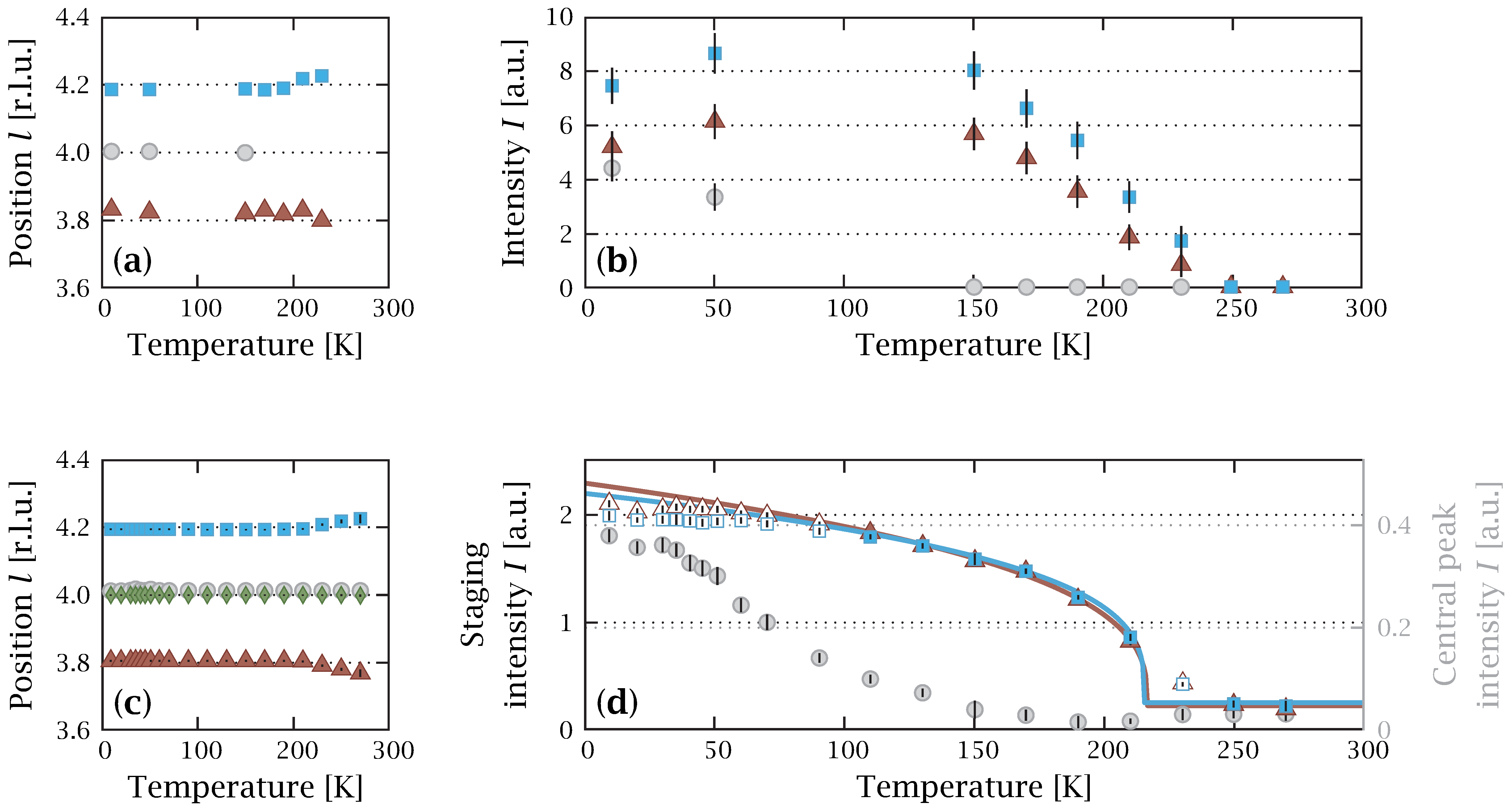
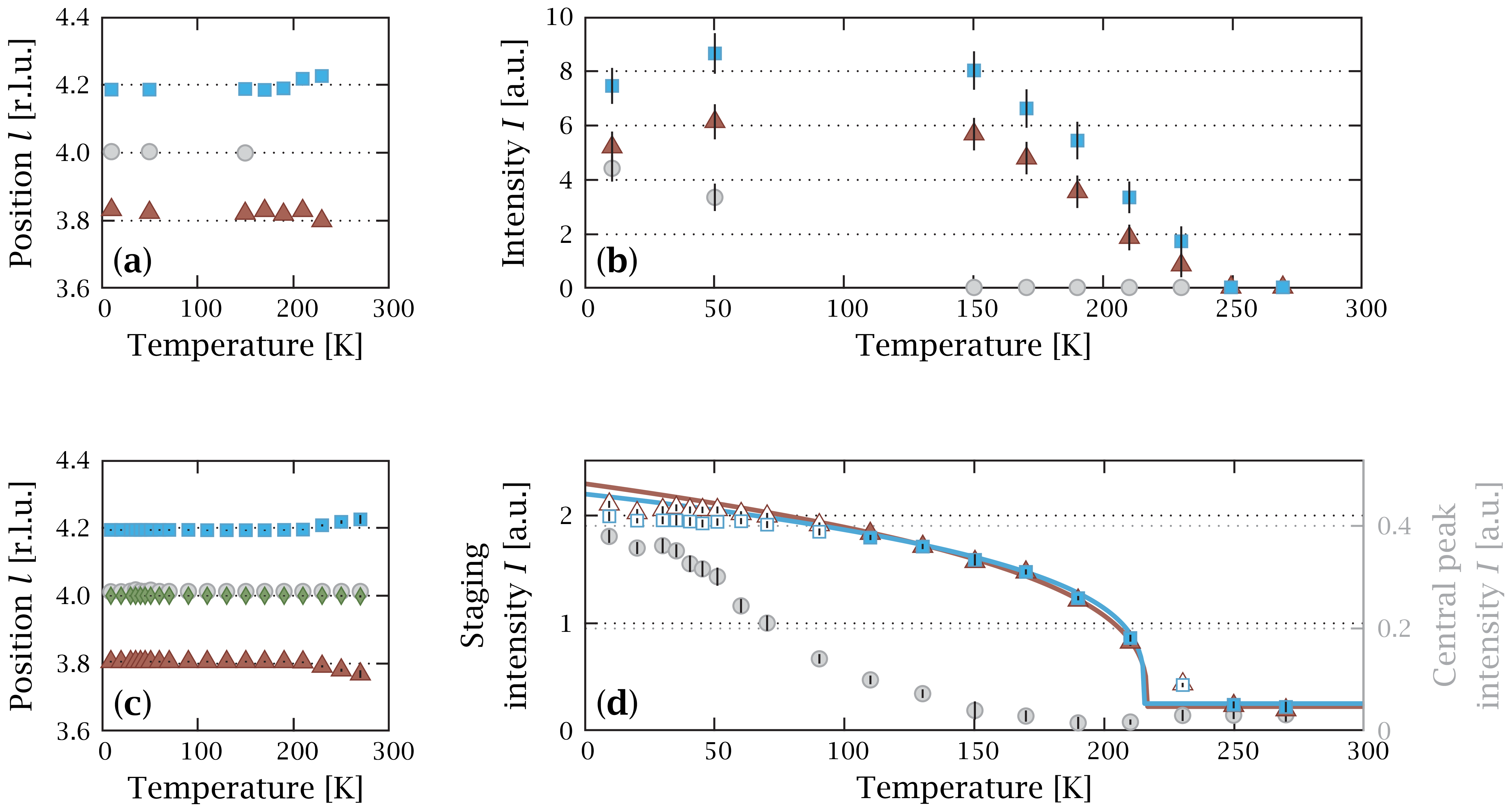
Figur 7.3: Peak positions and integrated intensities for the x = 0.04 sample. Download links:PNG • αPNG • SVG • PDF. .
DMC-illustrationer og dataplots (kapitel 8)
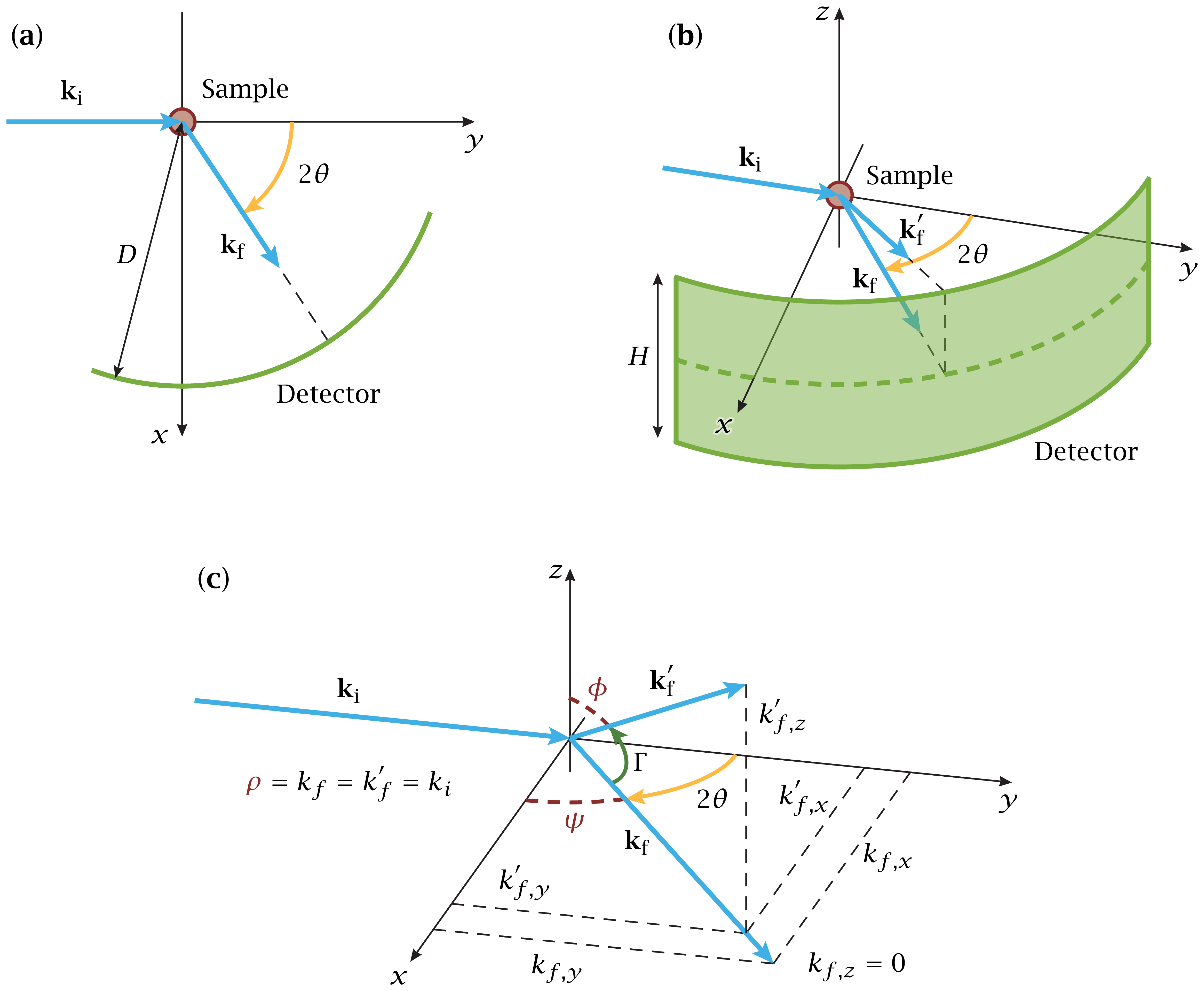
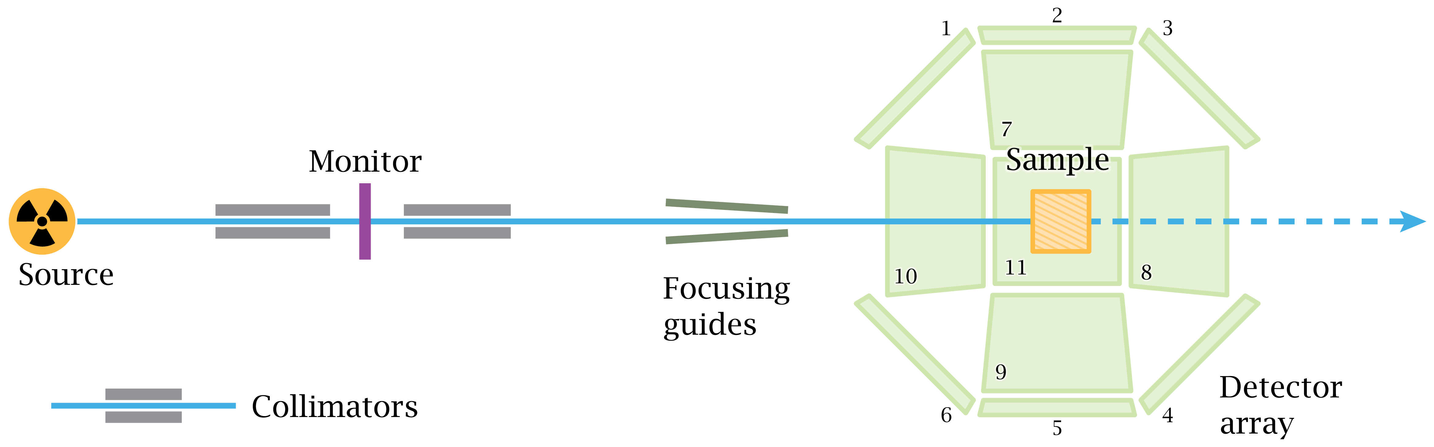
Figur 8.1: Overview sketch of the DMC instrument. Download links:PNG • αPNG • SVG • PDF. .
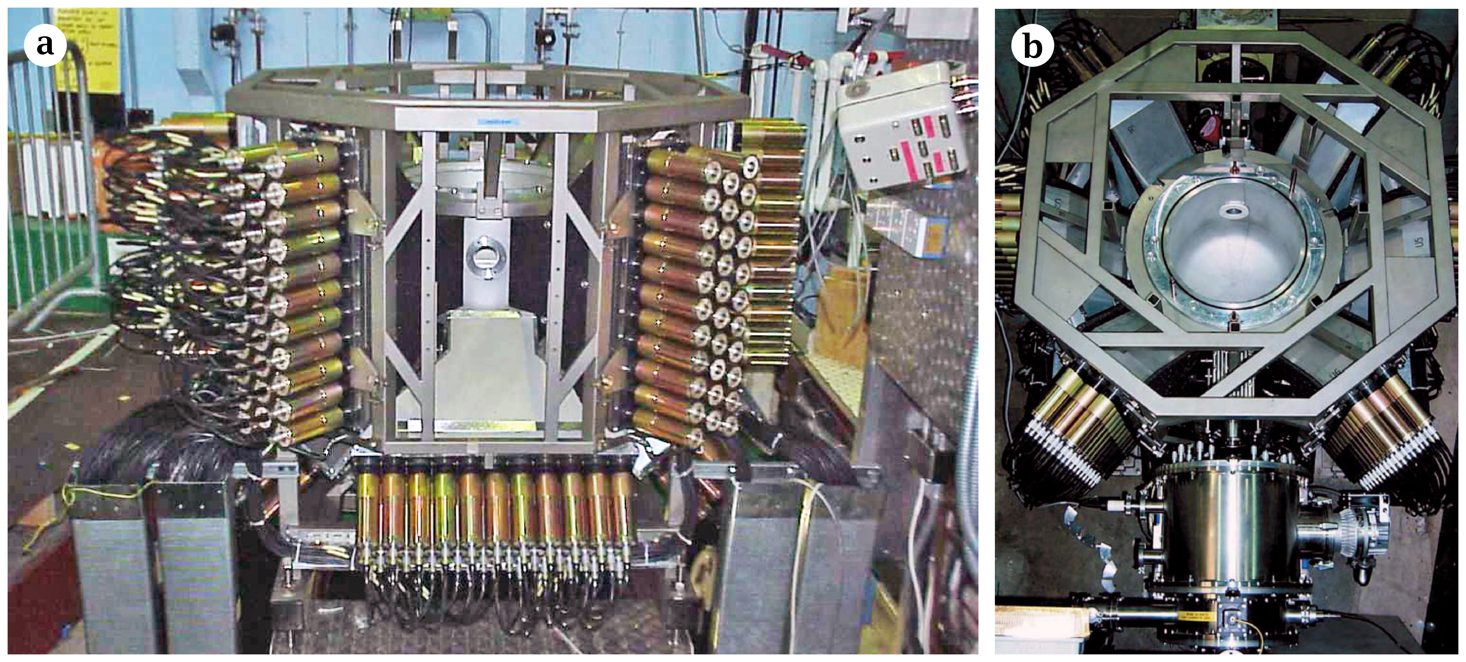
Figur 8.2: Photo of the DMC instrument. Download links:PNG • SVG • PDF. .
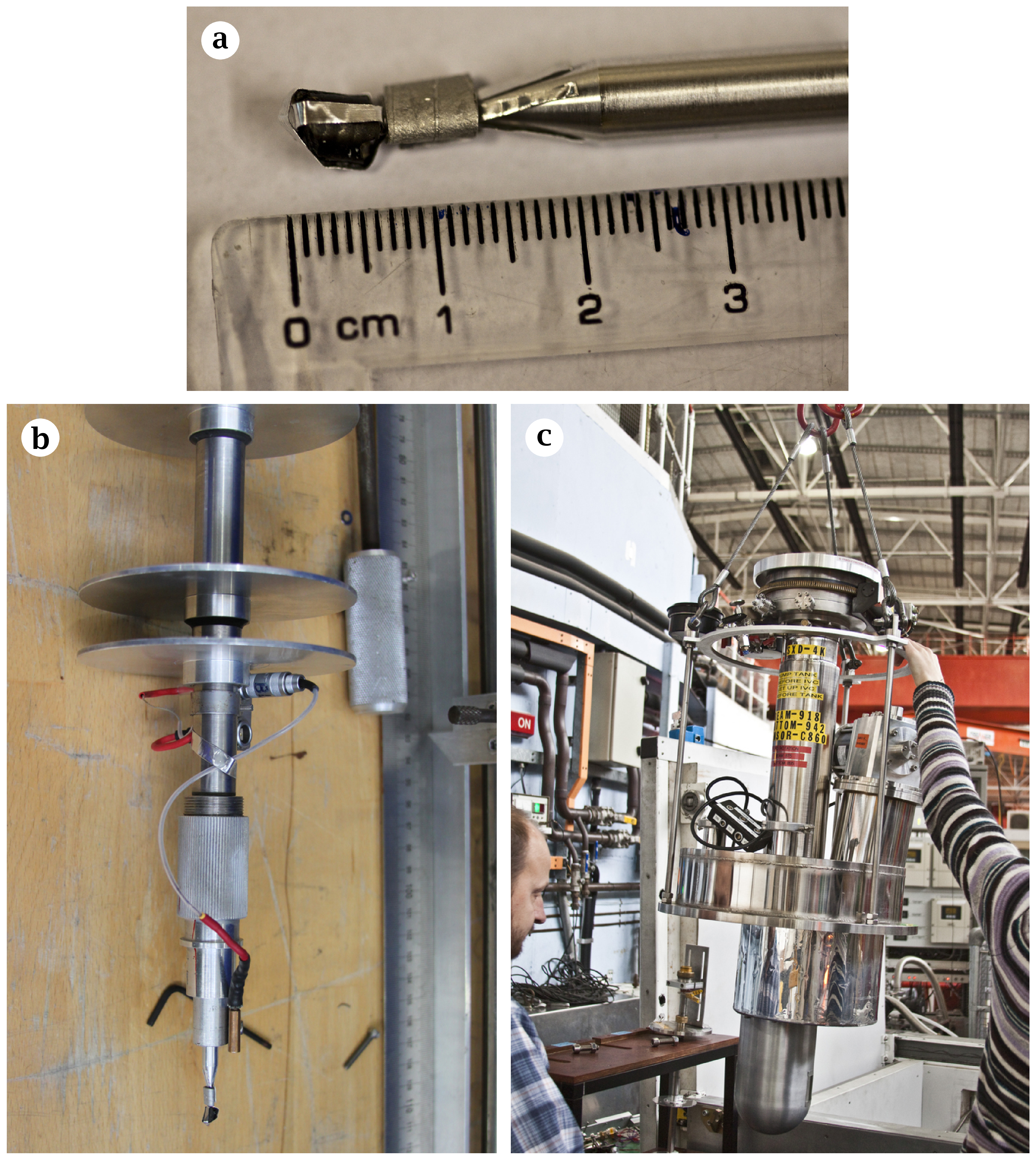
Figur 8.3: Photos of three of the samples measured on at DMC. Download links:PNG • αPNG • SVG • PDF. .
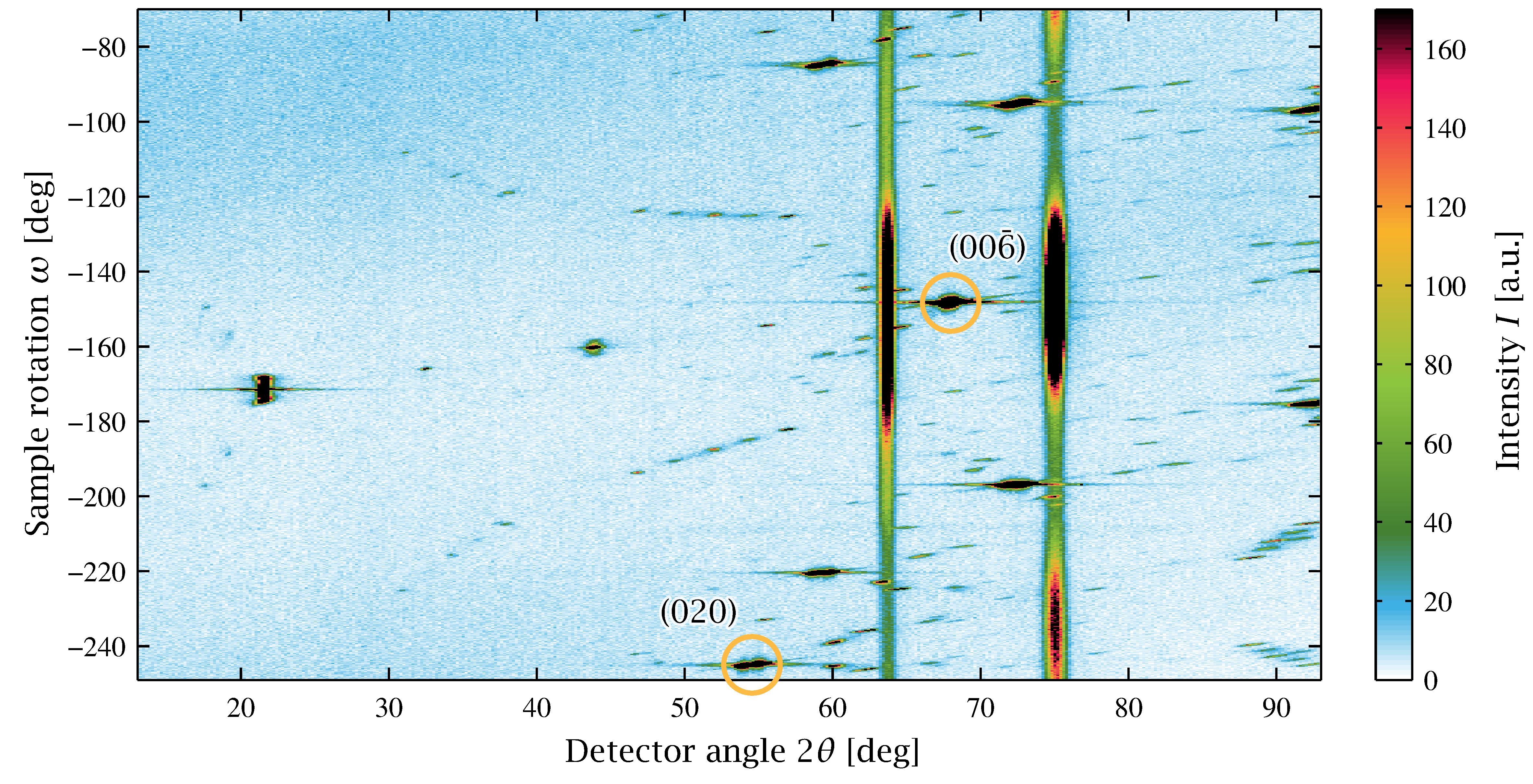
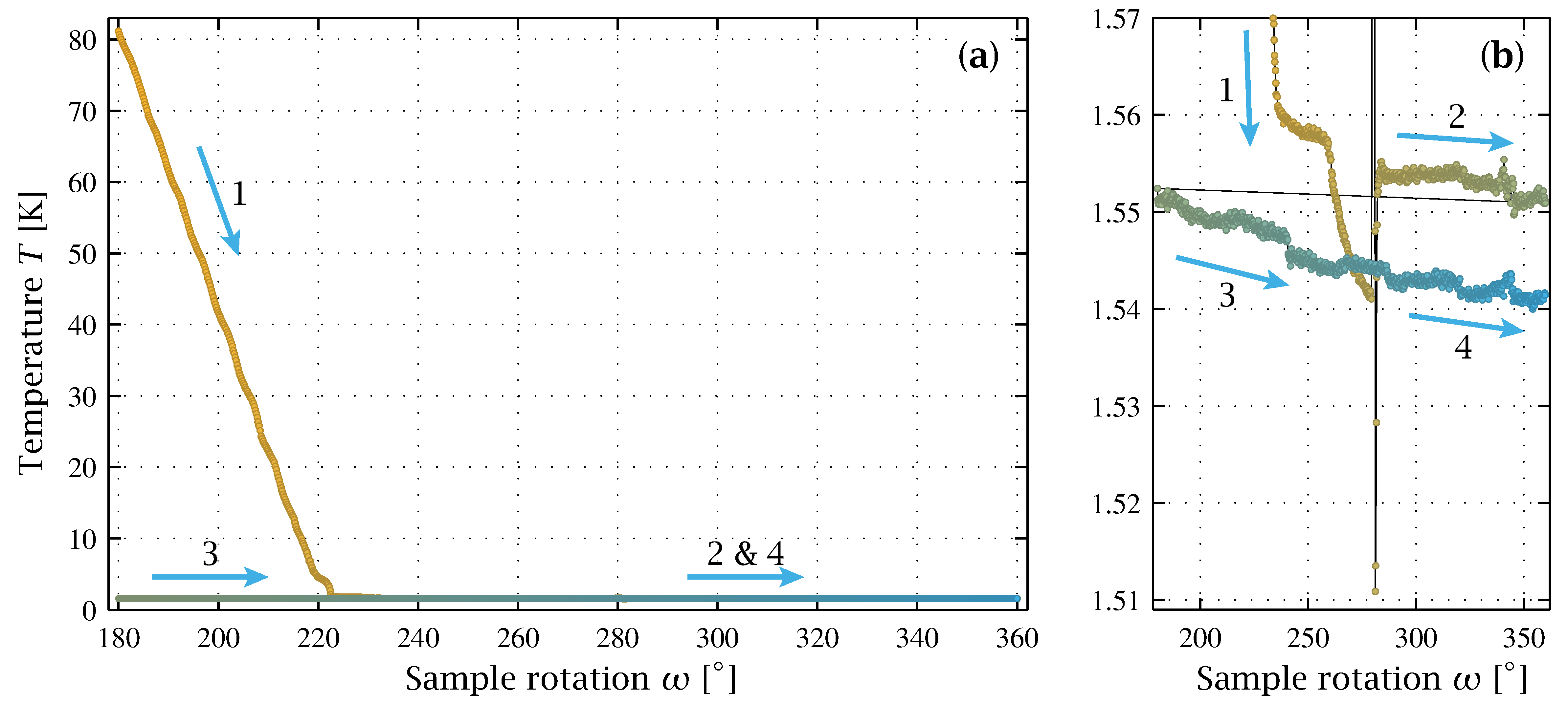
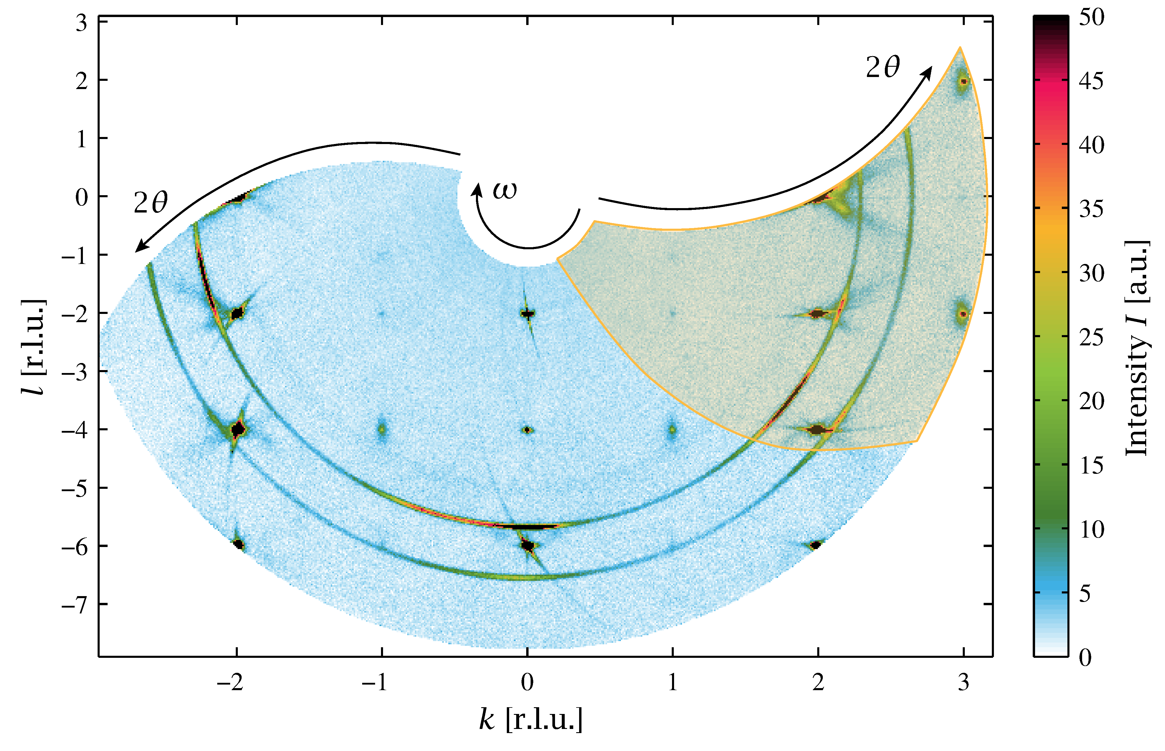
Figur 8.4: Example of (2θ,ω) plane for La(2)CuO(4+y). Download links:PNG • SVG • PDF. .
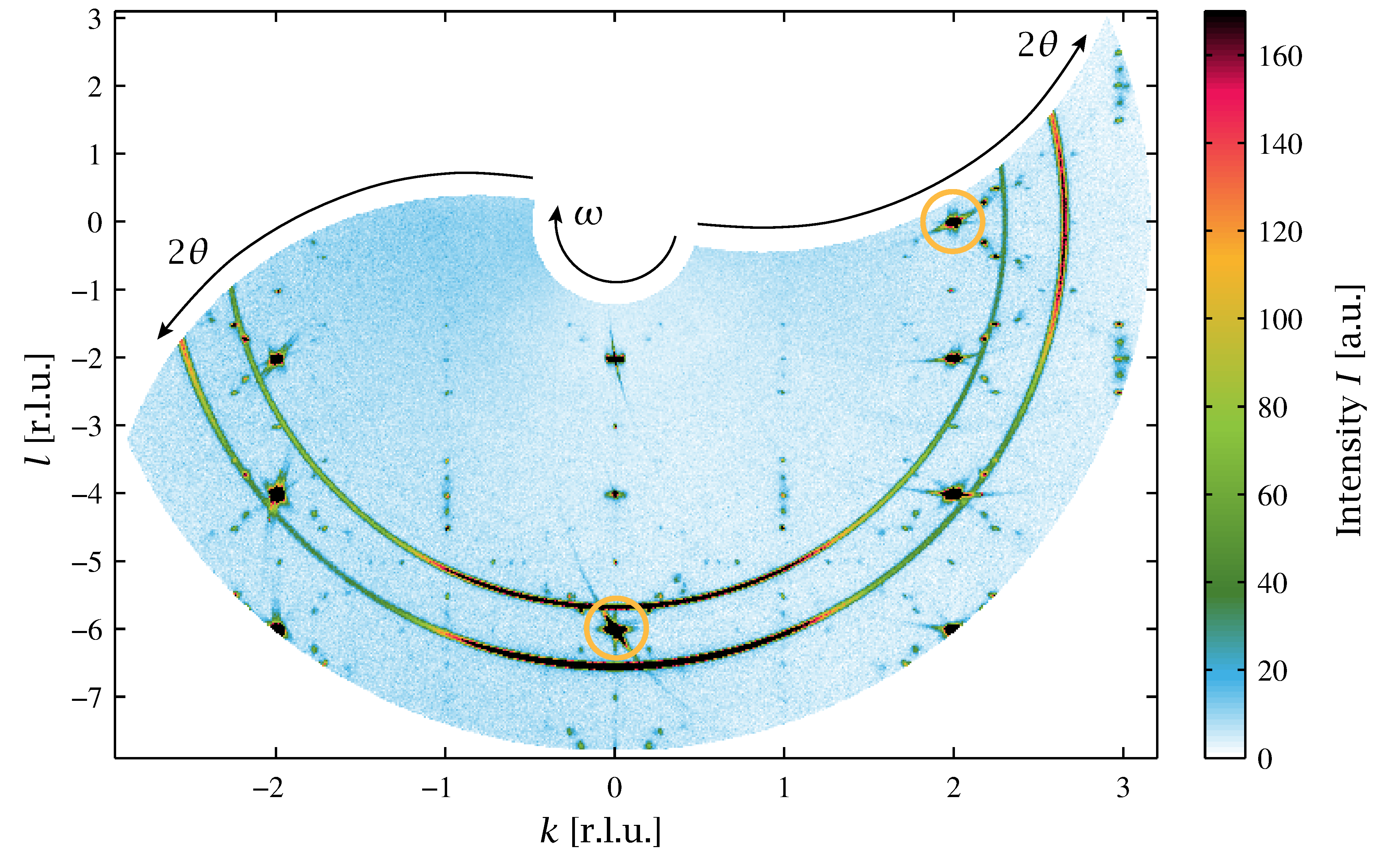
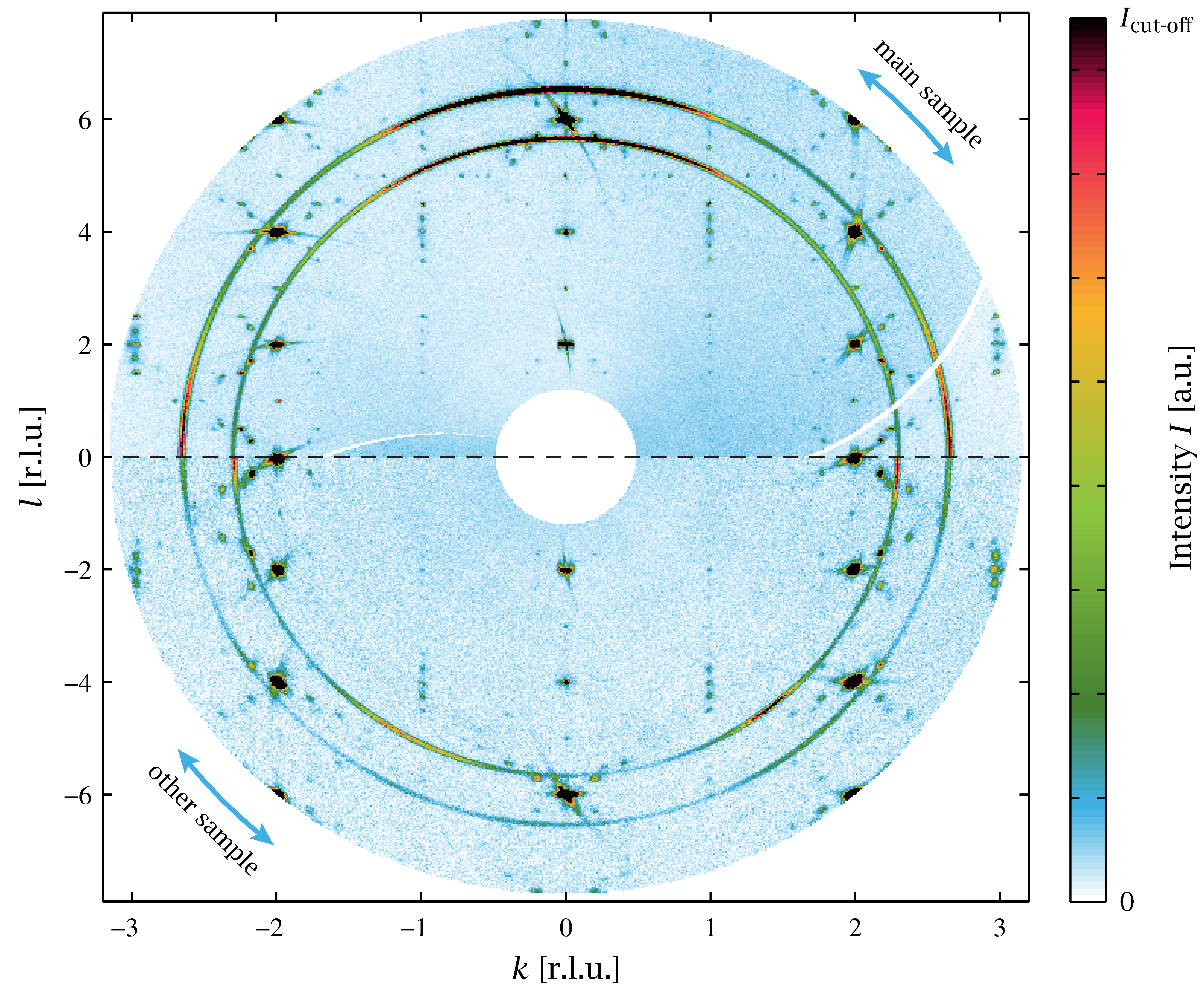
Figur 8.5: Example of a (0kl) reciprocal-space map for La(2)CuO(4+y). Download links:PNG • SVG • PDF. .
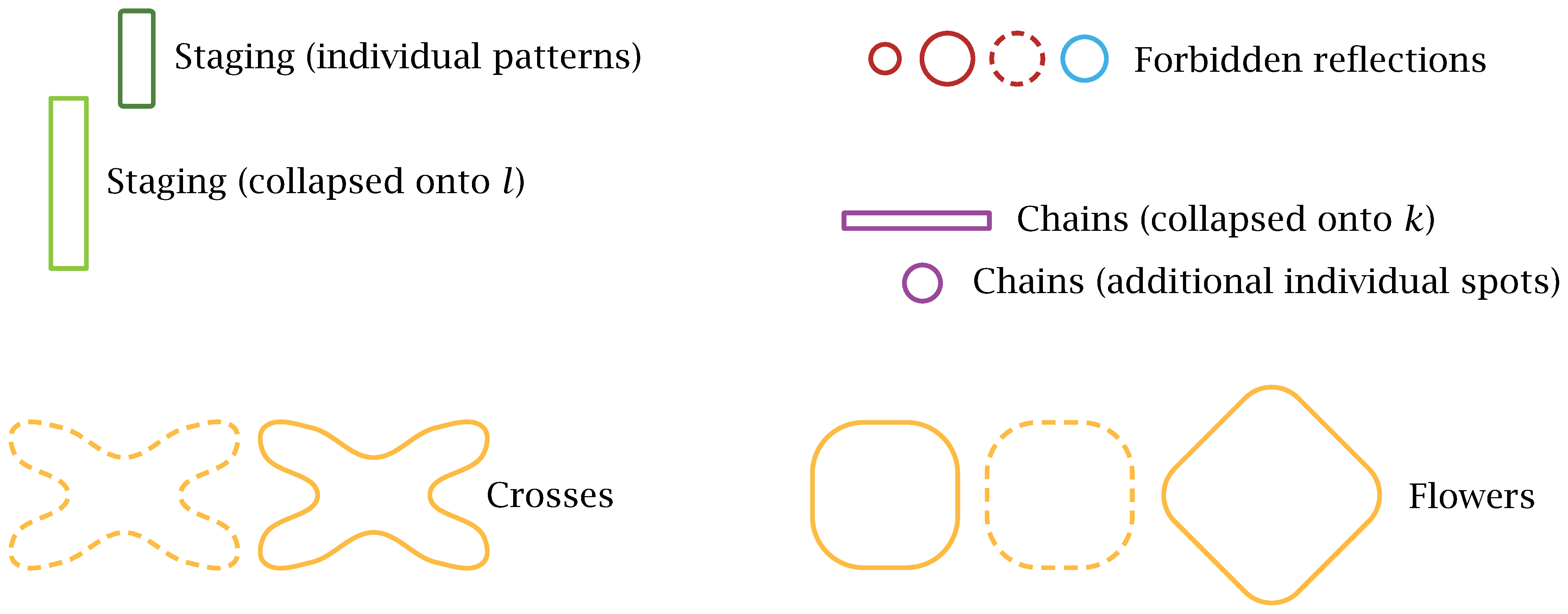
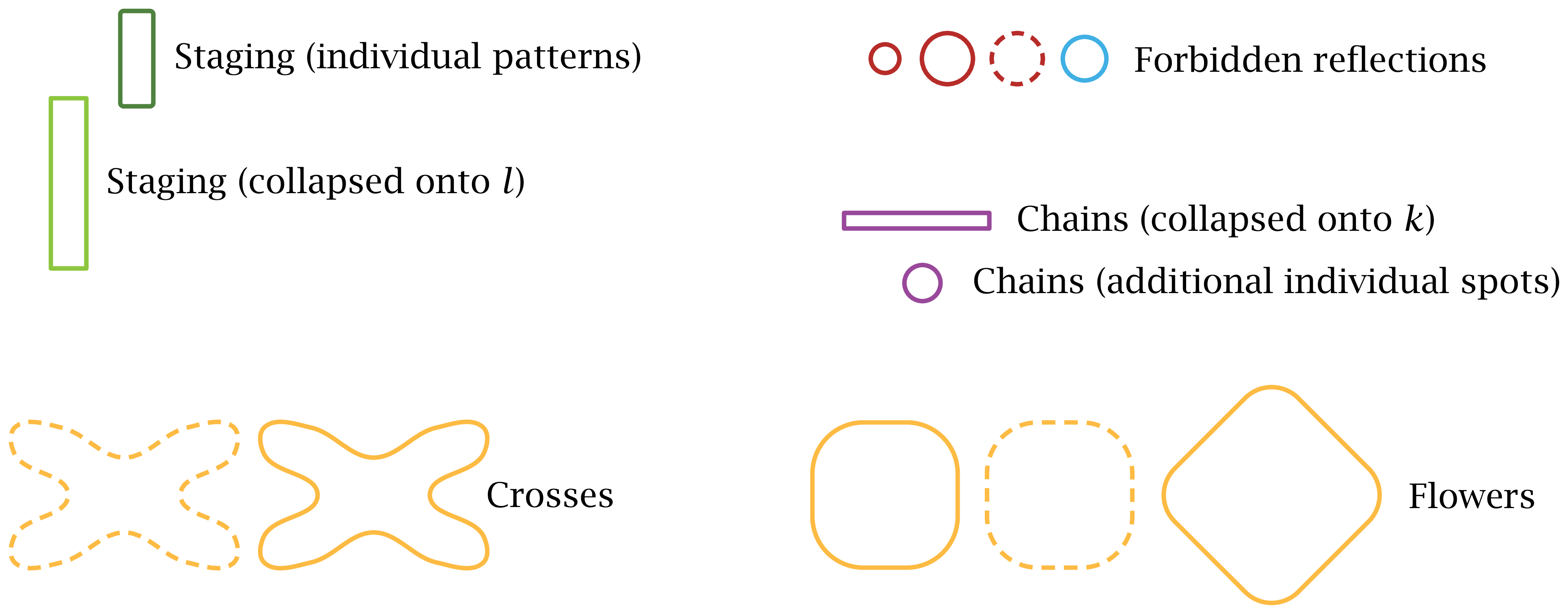
Figur 8.6: Types of annotation markers used in the DMC reciprocal-space planes. Download links:PNG • αPNG • SVG • PDF. .
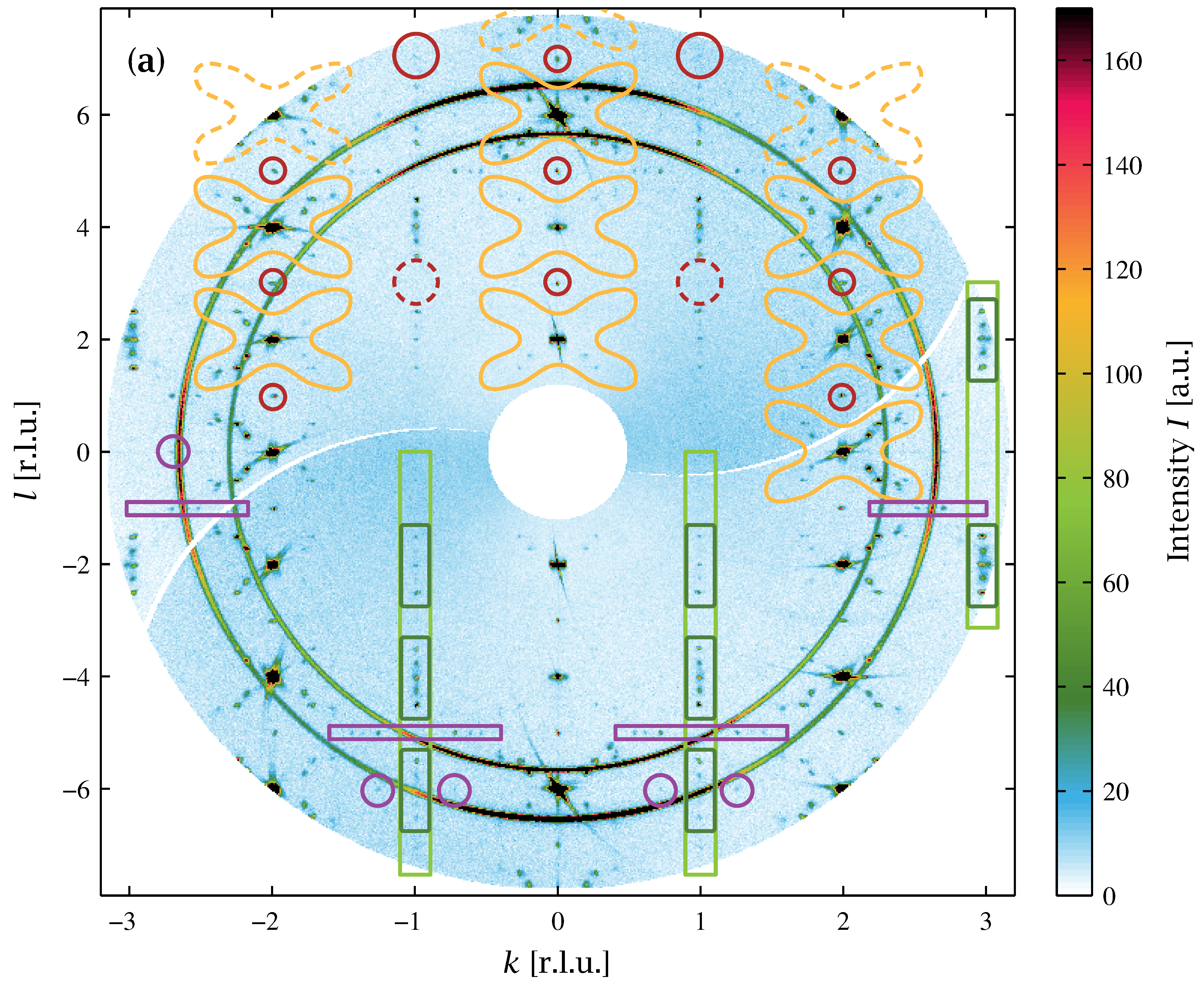
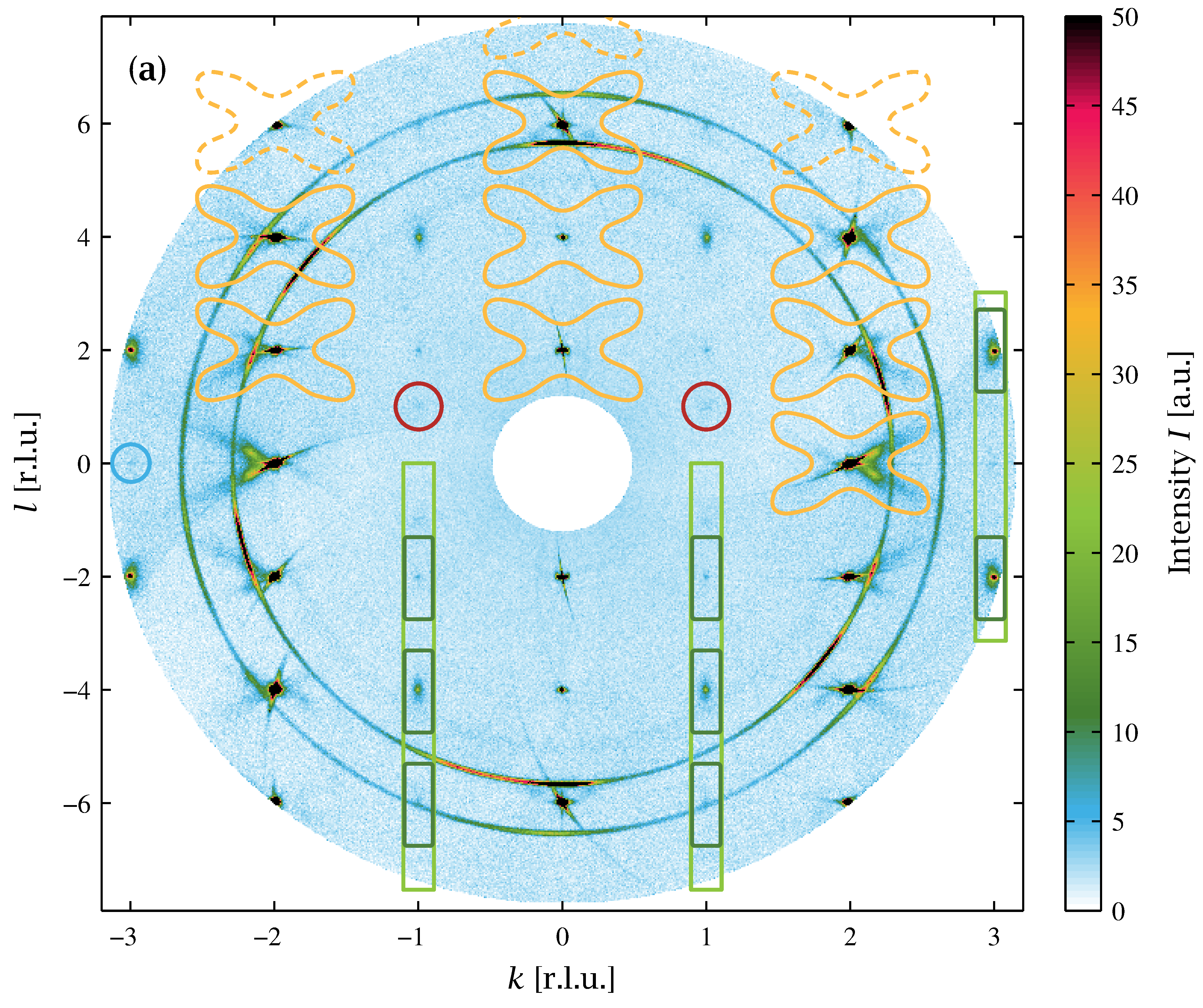
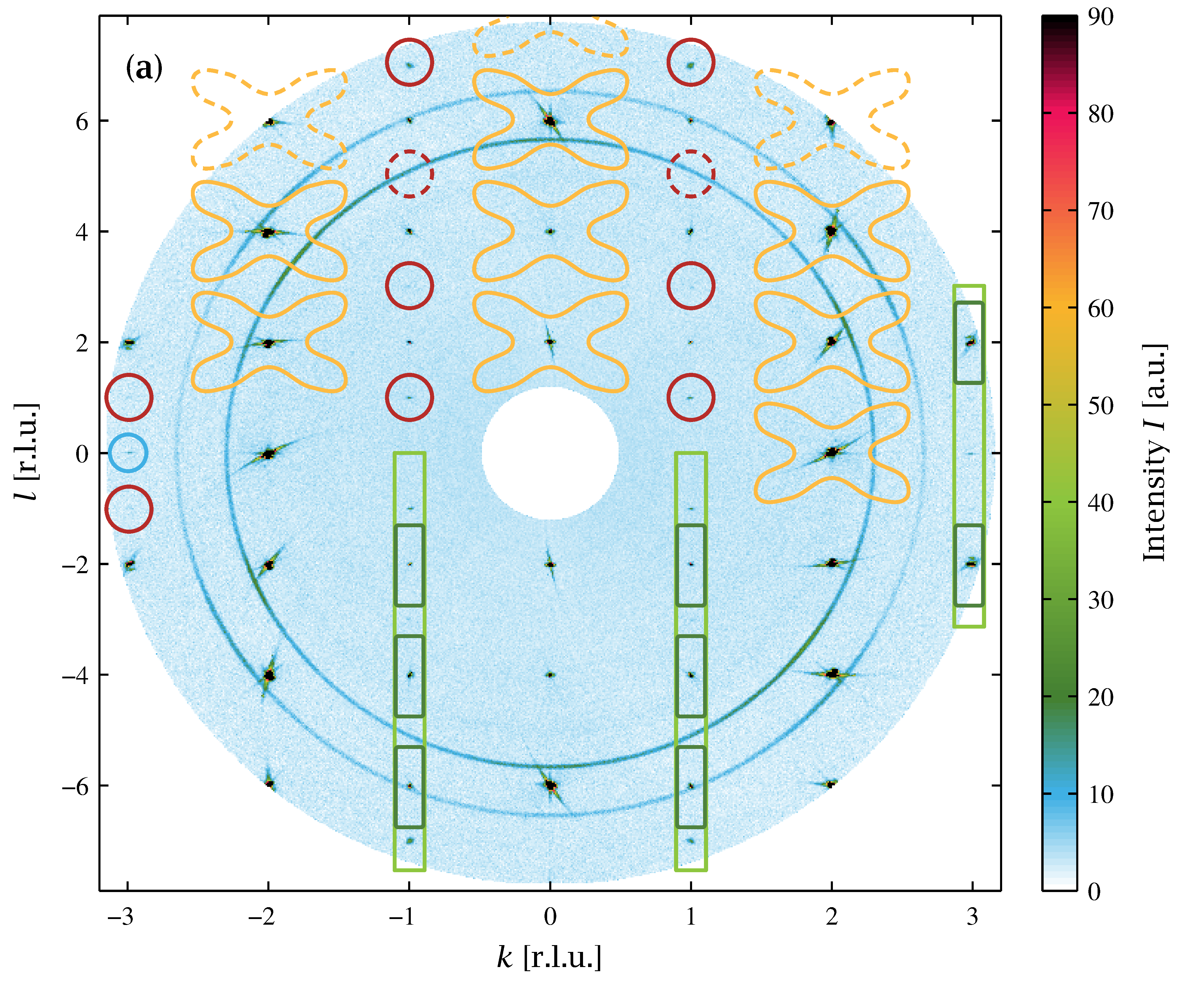
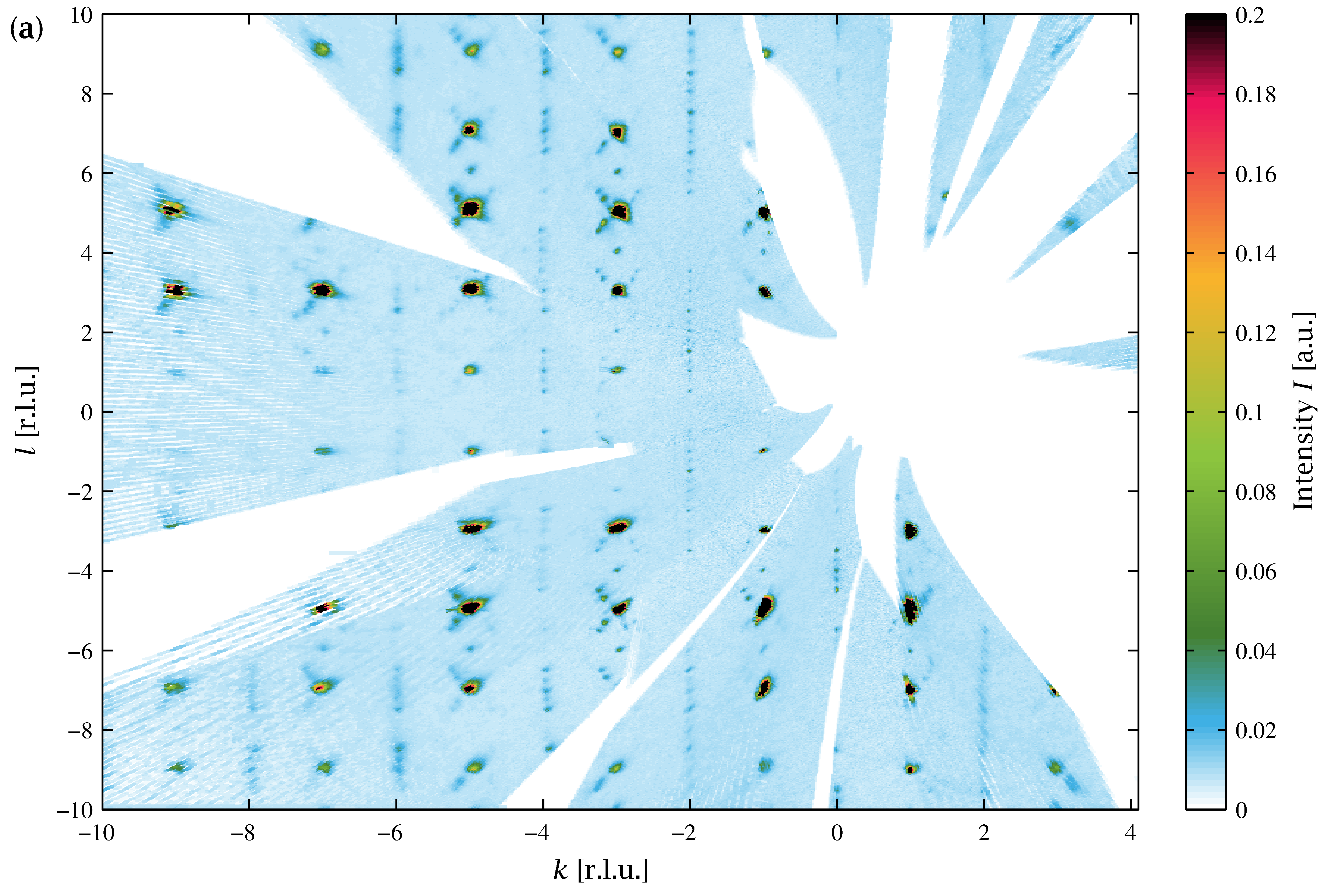
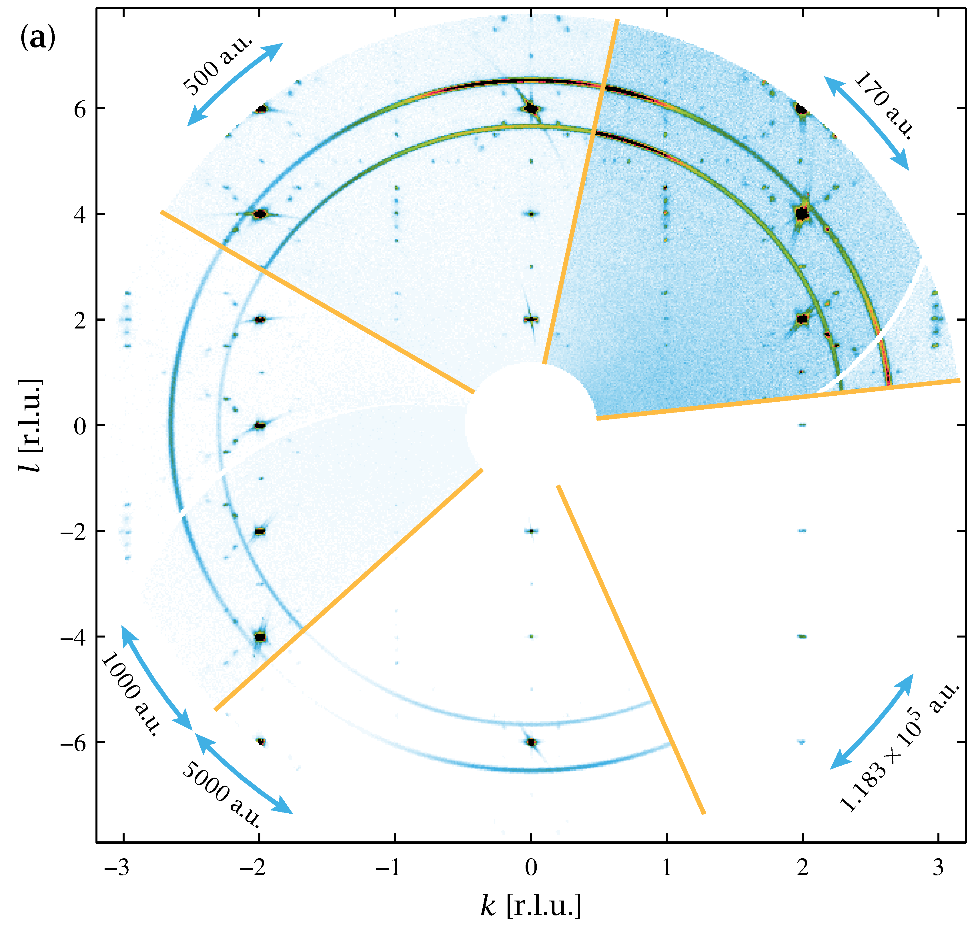
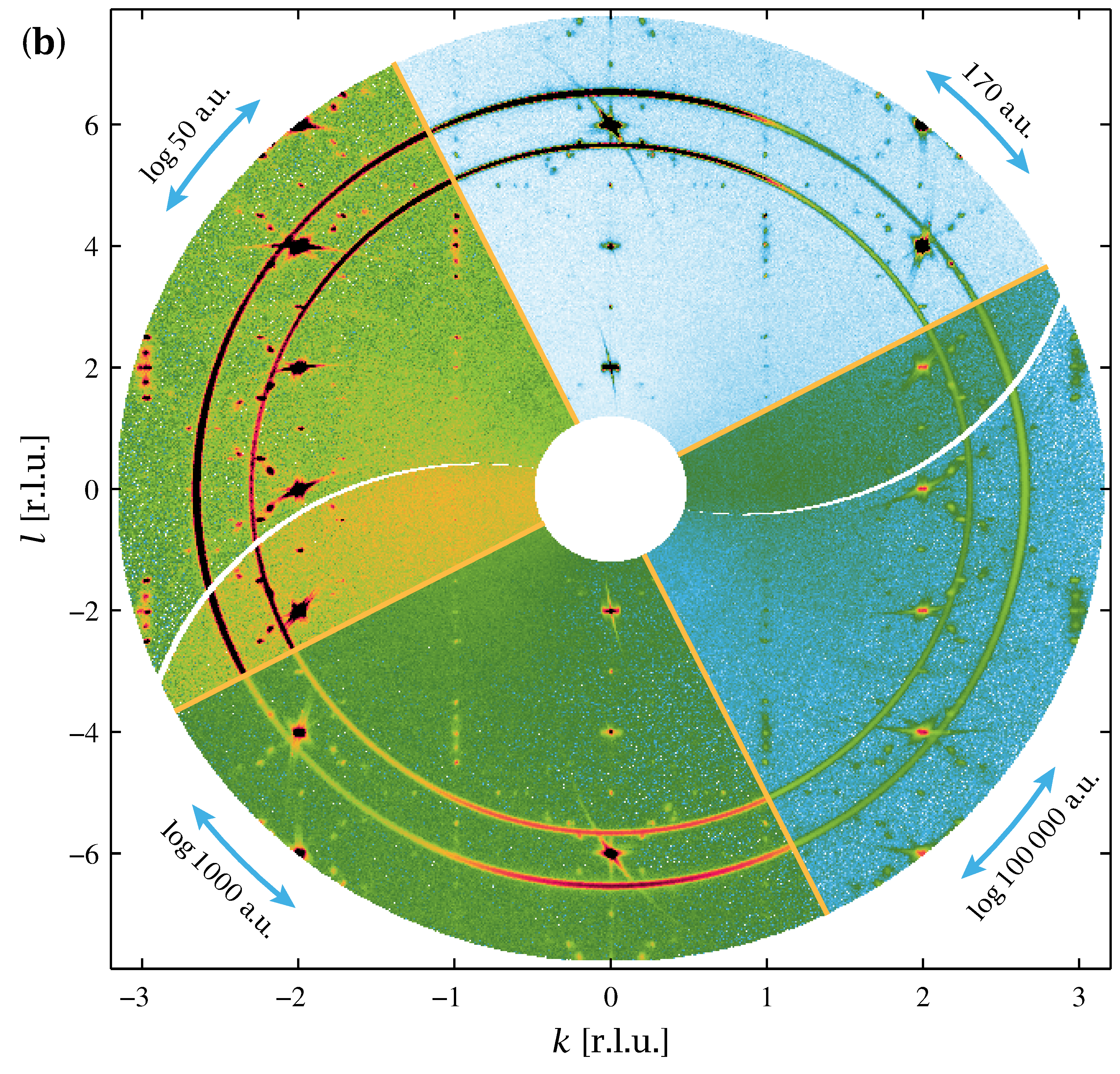
Figur 8.7(a): Low-temperature reciprocal-space (0kl) map for the La(2)CuO(4+y) sample. Download links:PNG • SVG • PDF. .
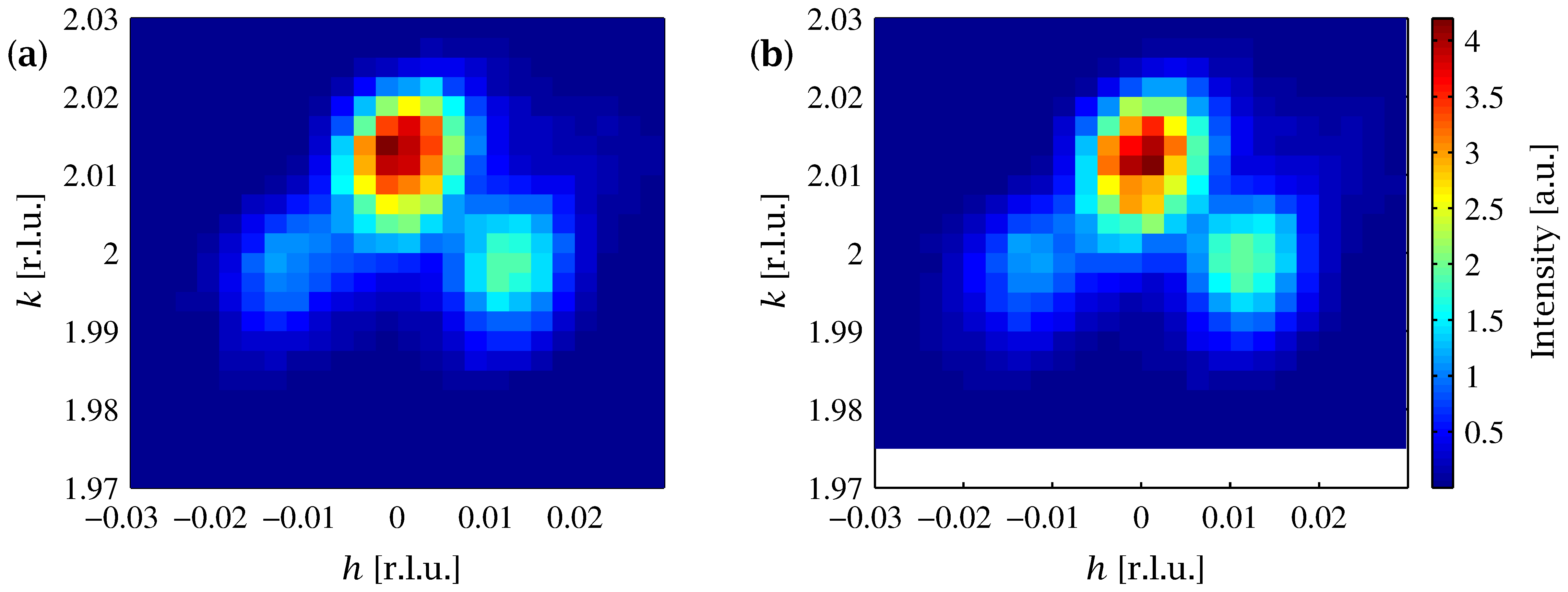
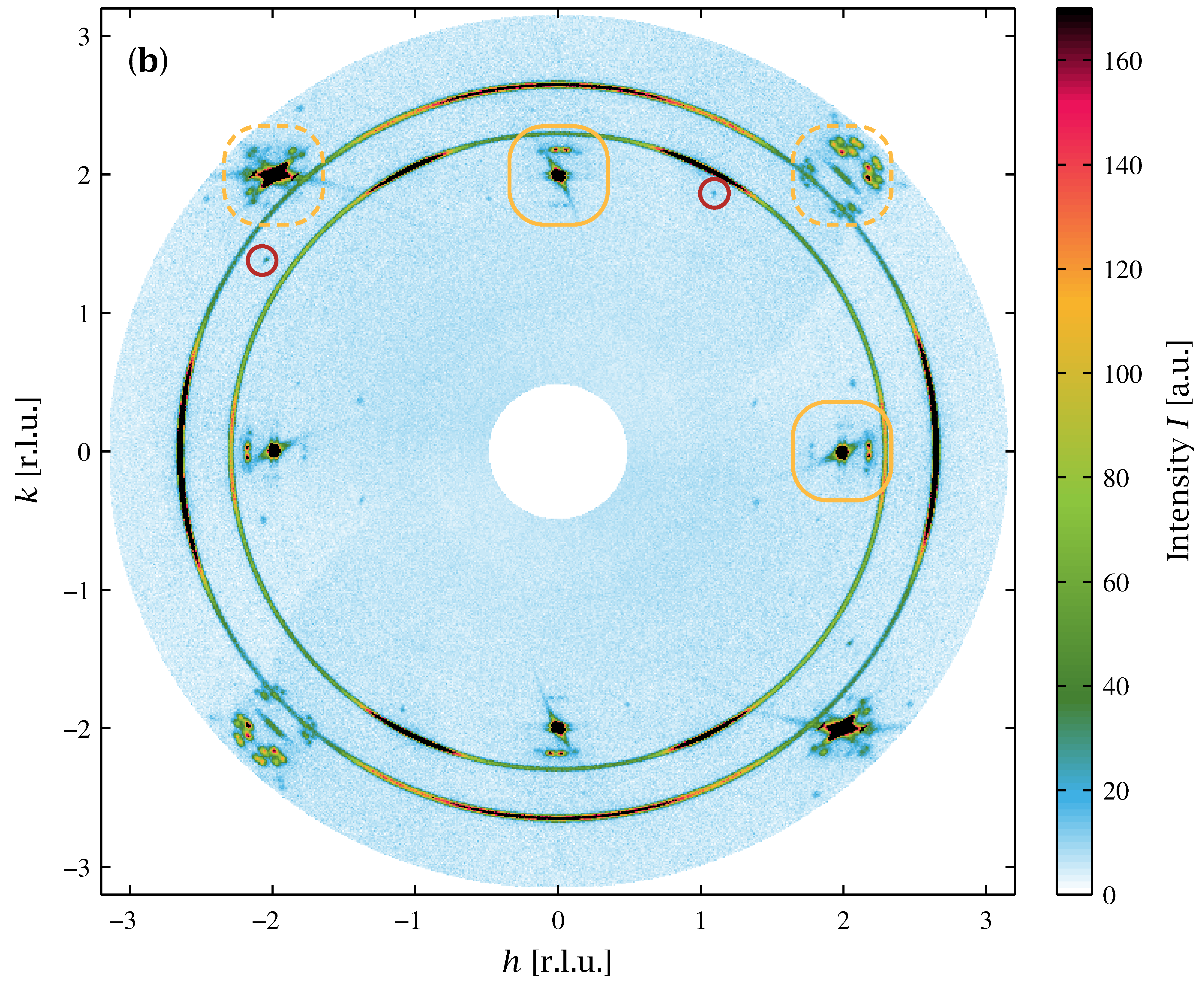
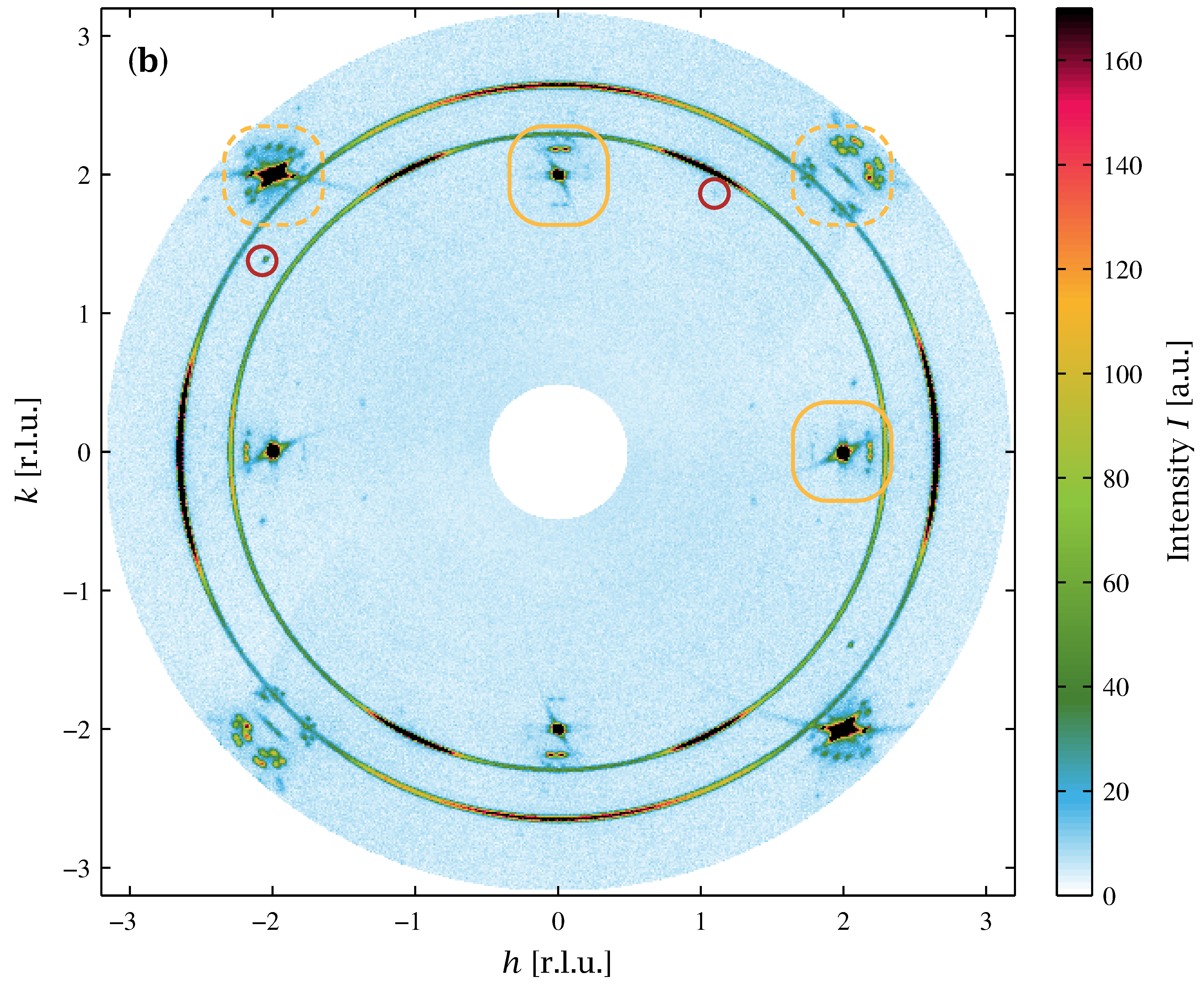
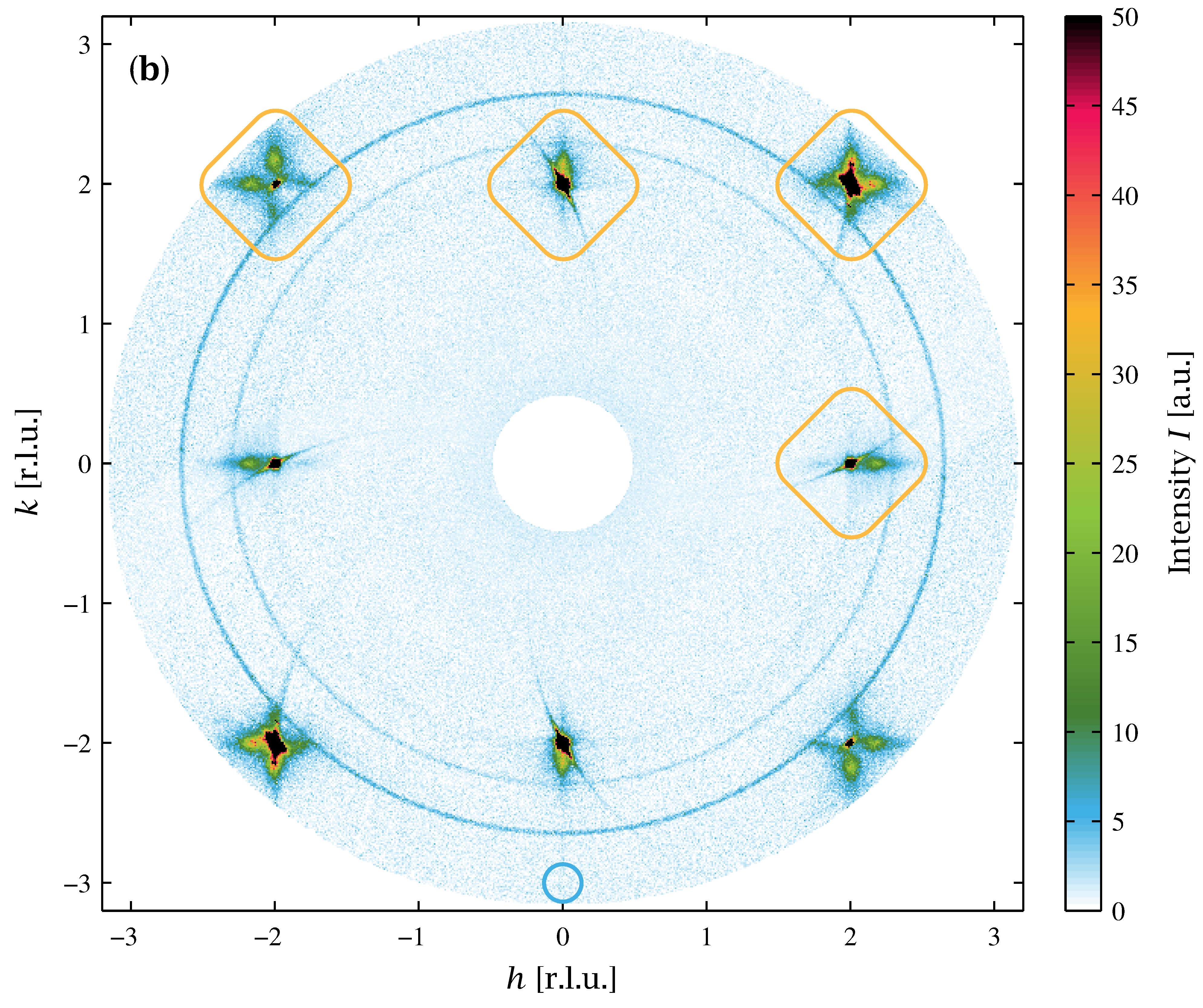
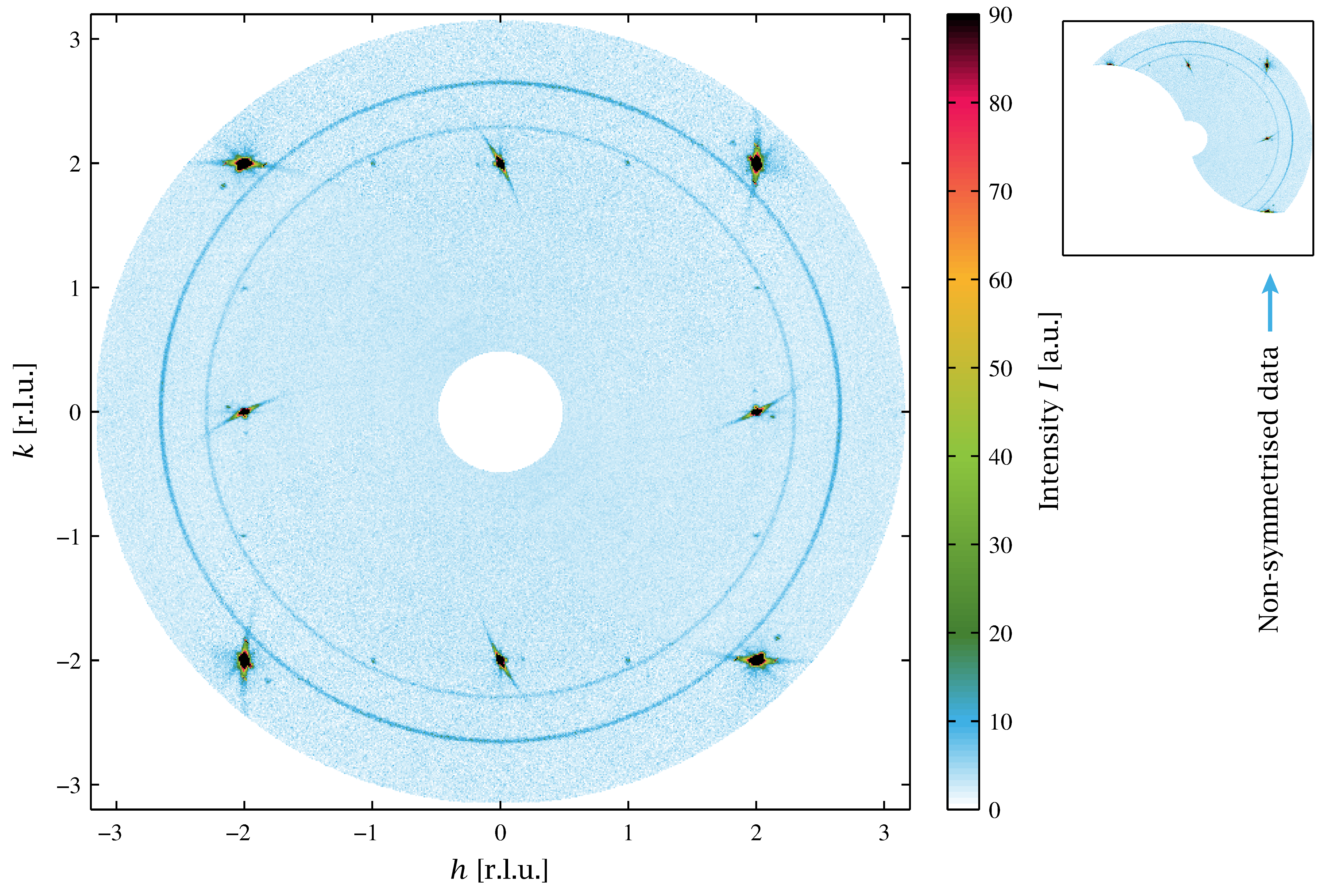
Figur 8.7(b): Low-temperature reciprocal-space (hk0) map for the La(2)CuO(4+y) sample. Download links:PNG • SVG • PDF. .
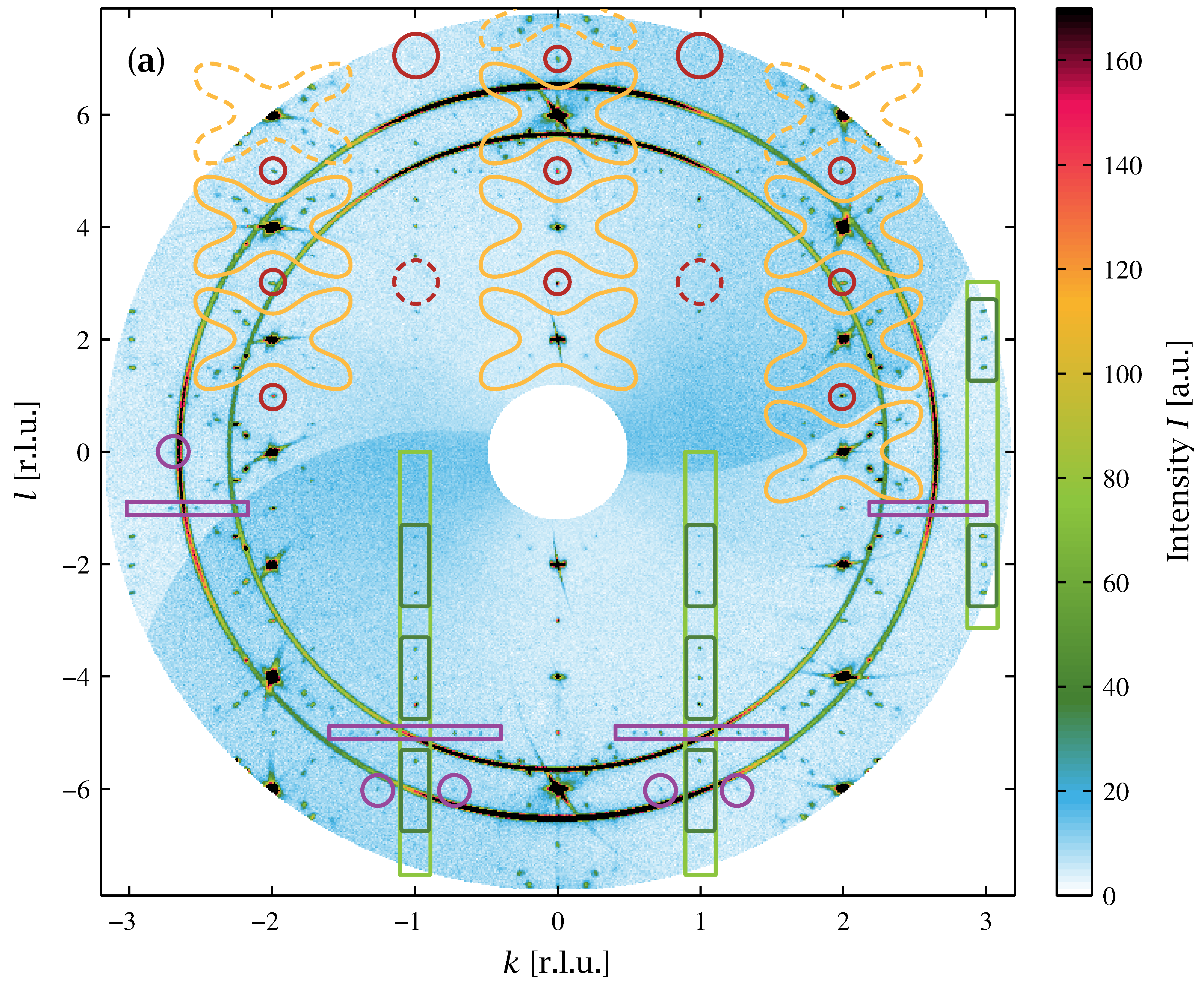
Figur 8.8(a): Room-temperature reciprocal-space (0kl) map for the La(2)CuO(4+y) sample. Download links:PNG • SVG • PDF. .
Figur 8.8(b): Room-temperature reciprocal-space (hk0) map for the La(2)CuO(4+y) sample. Download links:PNG • SVG • PDF. .
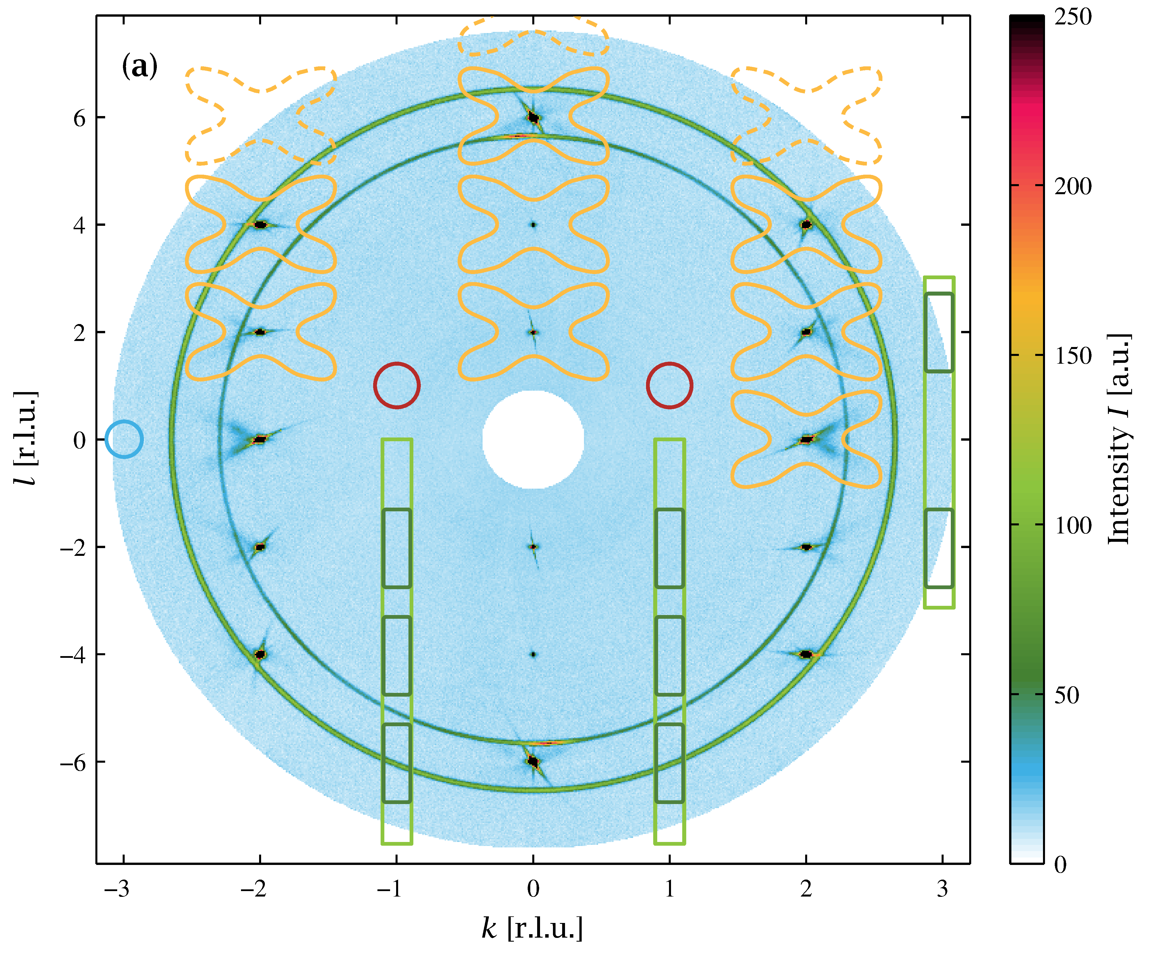
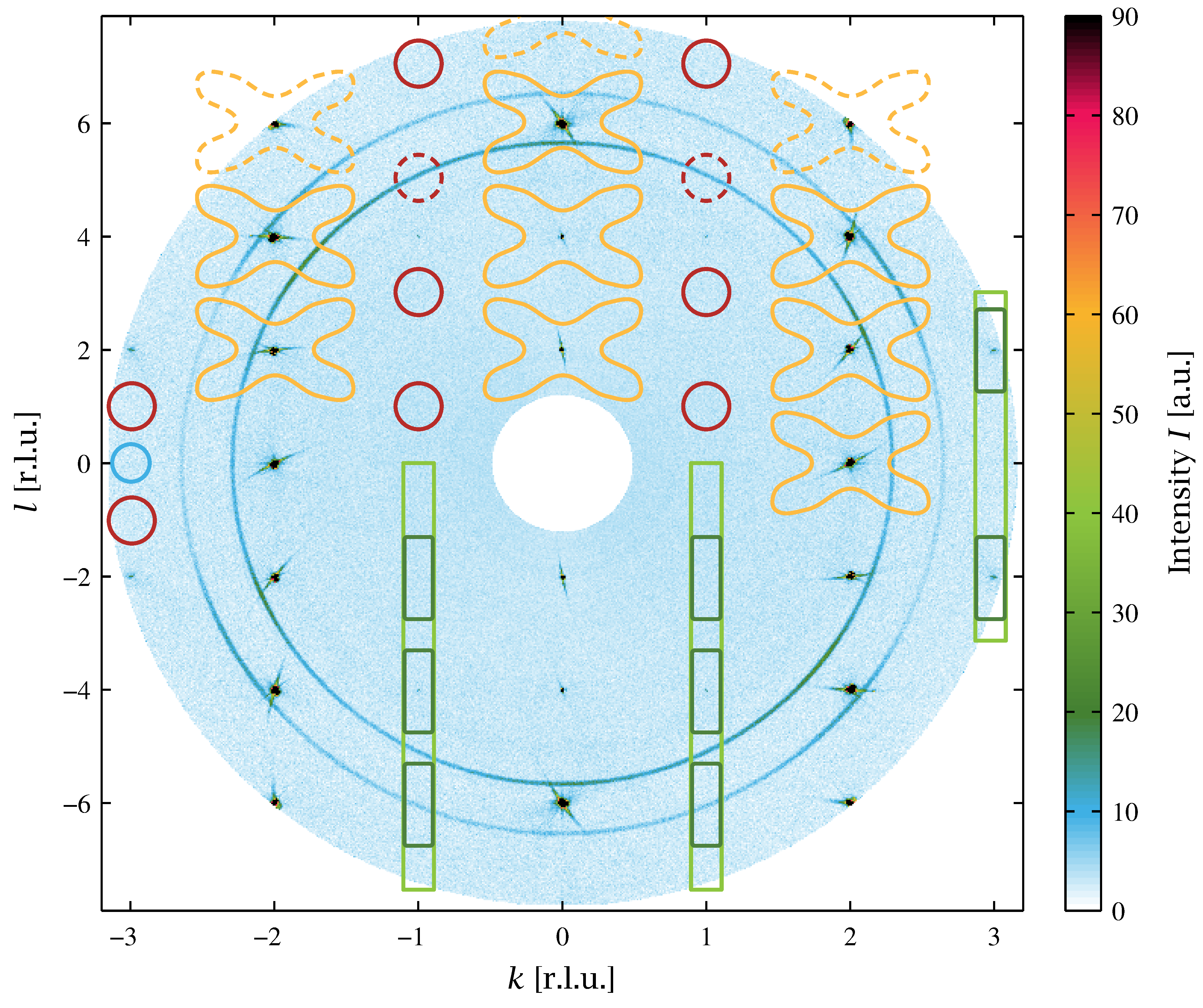
Figur 8.9(a): Low-temperature reciprocal-space (0kl) map for the La(1.94)Sr(0.06)CuO(4+y) sample. Download links:PNG • SVG • PDF. .
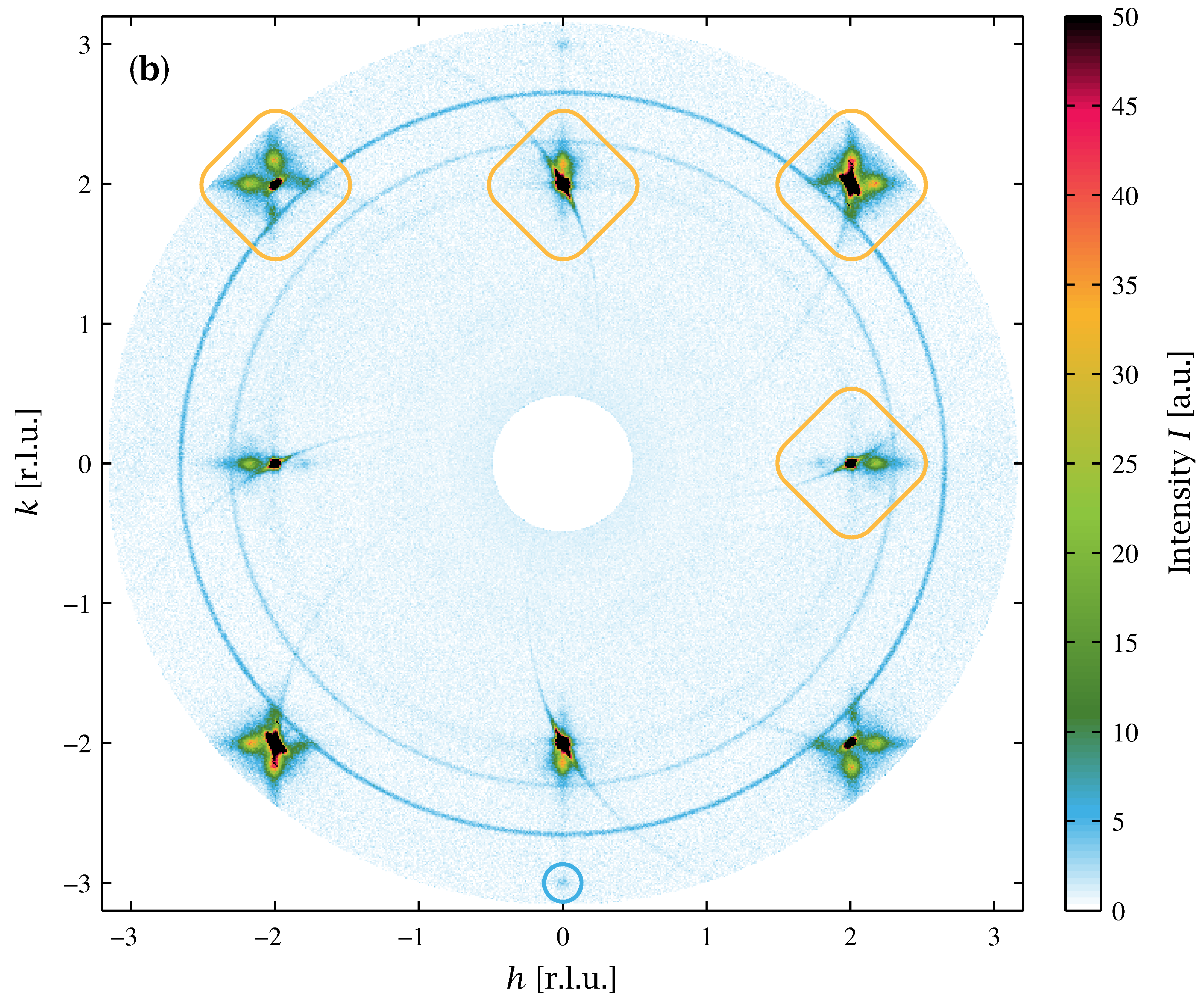
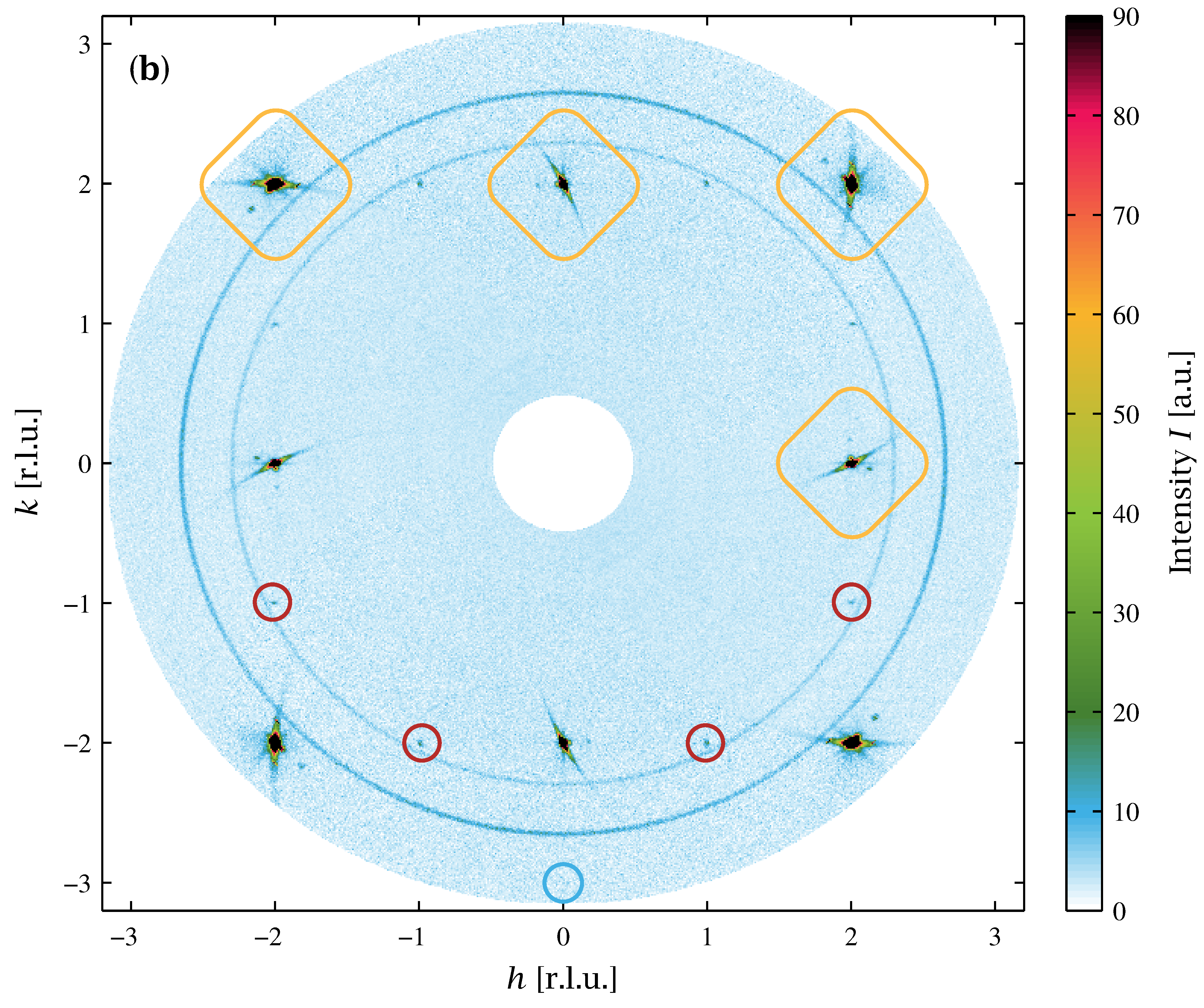
Figur 8.9(b): Low-temperature reciprocal-space (hk0) map for the La(1.94)Sr(0.06)CuO(4+y) sample. Download links:PNG • SVG • PDF. .
Figur 8.10(a): Room-temperature reciprocal-space (0kl) map for the La(1.94)Sr(0.06)CuO(4+y) sample. Download links:PNG • SVG • PDF. .
Figur 8.10(b): Room-temperature reciprocal-space (hk0) map for the La(1.94)Sr(0.06)CuO(4+y) sample. Download links:PNG • SVG • PDF. .
Figur 8.11(a): Mid-temperature reciprocal-space (0kl) map for the La(1.91)Sr(0.09)CuO(4+y) sample. Download links:PNG • SVG • PDF. .
Figur 8.11(b): Mid-temperature reciprocal-space (hk0) map for the La(1.91)Sr(0.09)CuO(4+y) sample. Download links:PNG • SVG • PDF. .
Figur 8.12: Room-temperature reciprocal-space (0kl) map for the La(1.91)Sr(0.09)CuO(4+y) sample. Download links:PNG • SVG • PDF. .
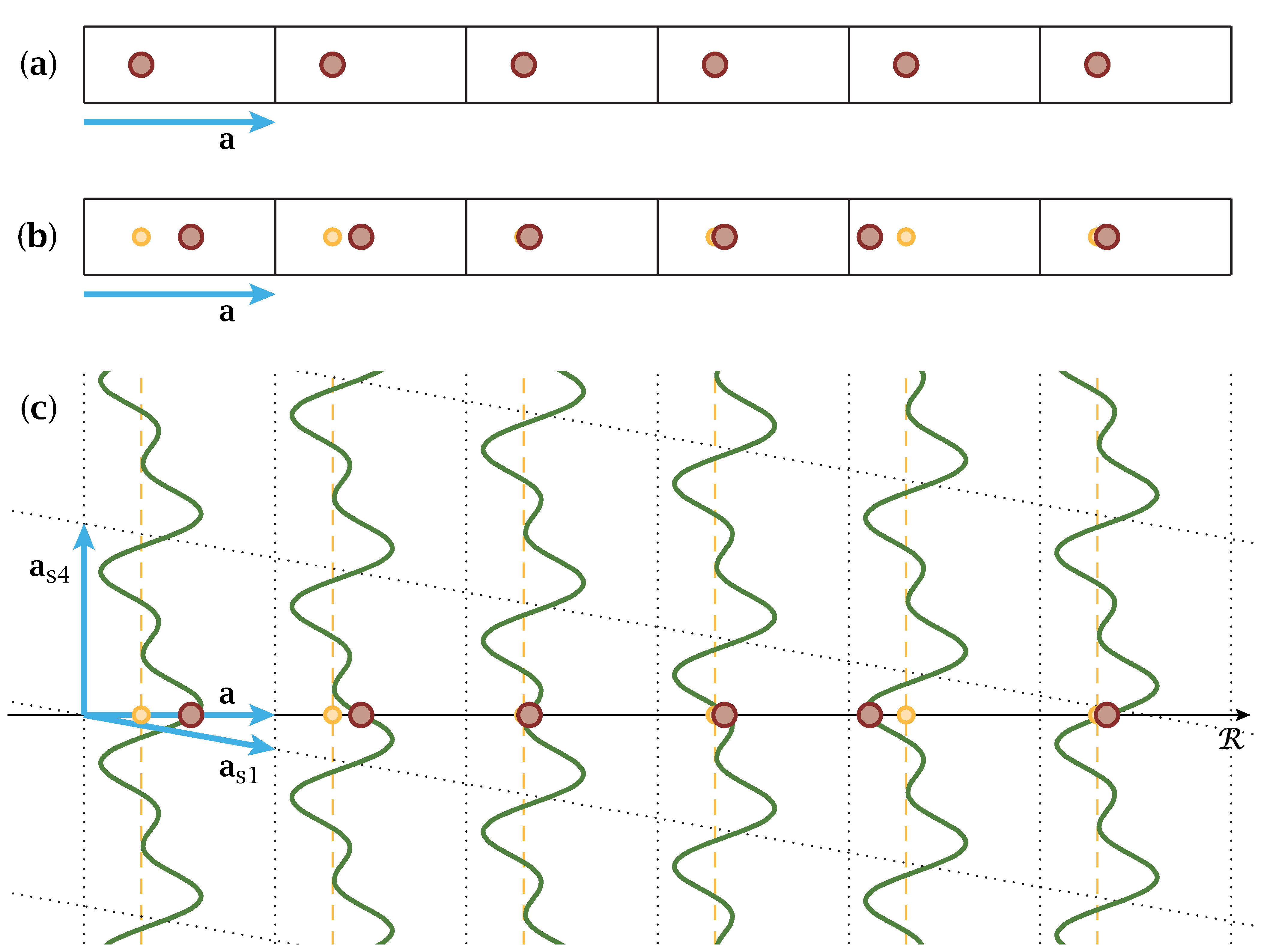
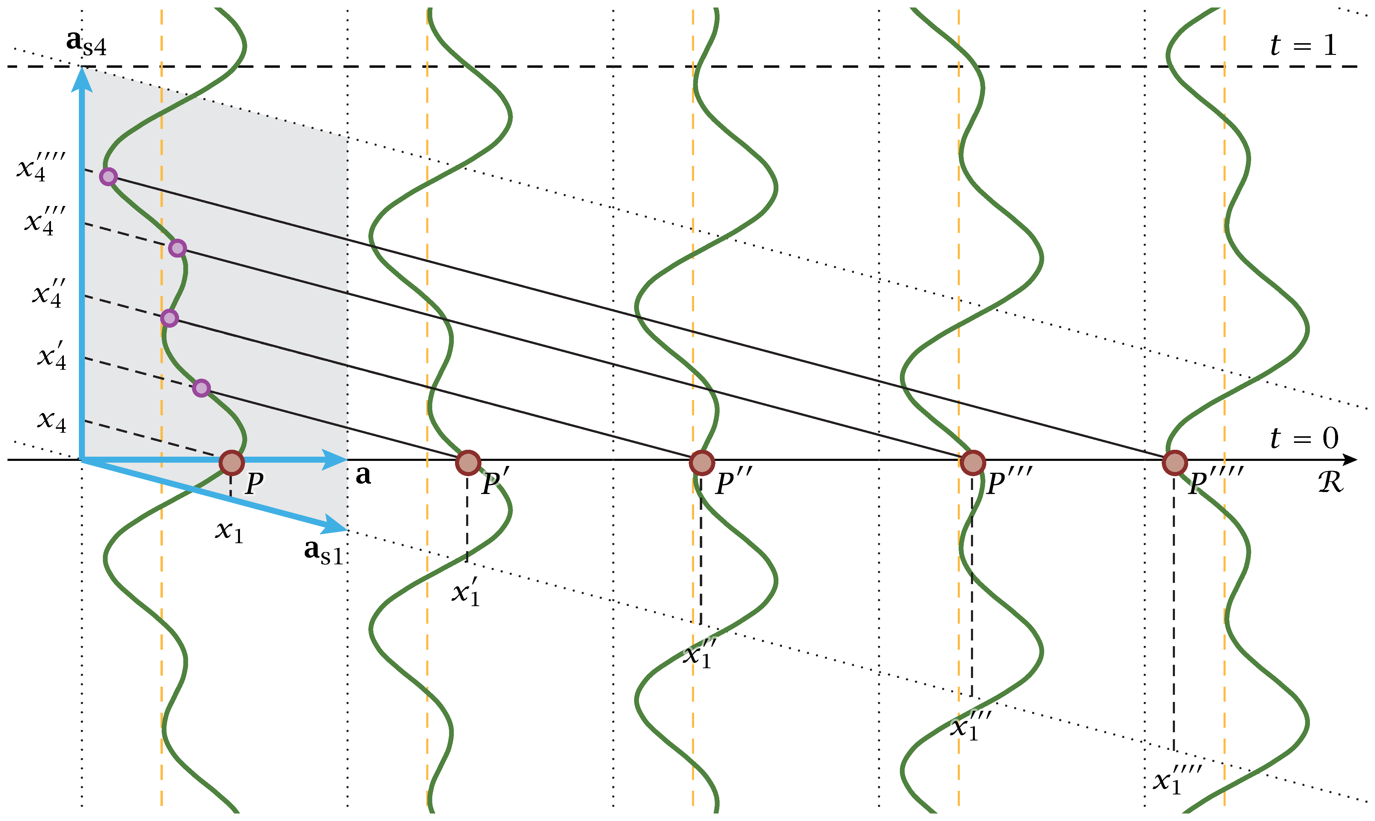
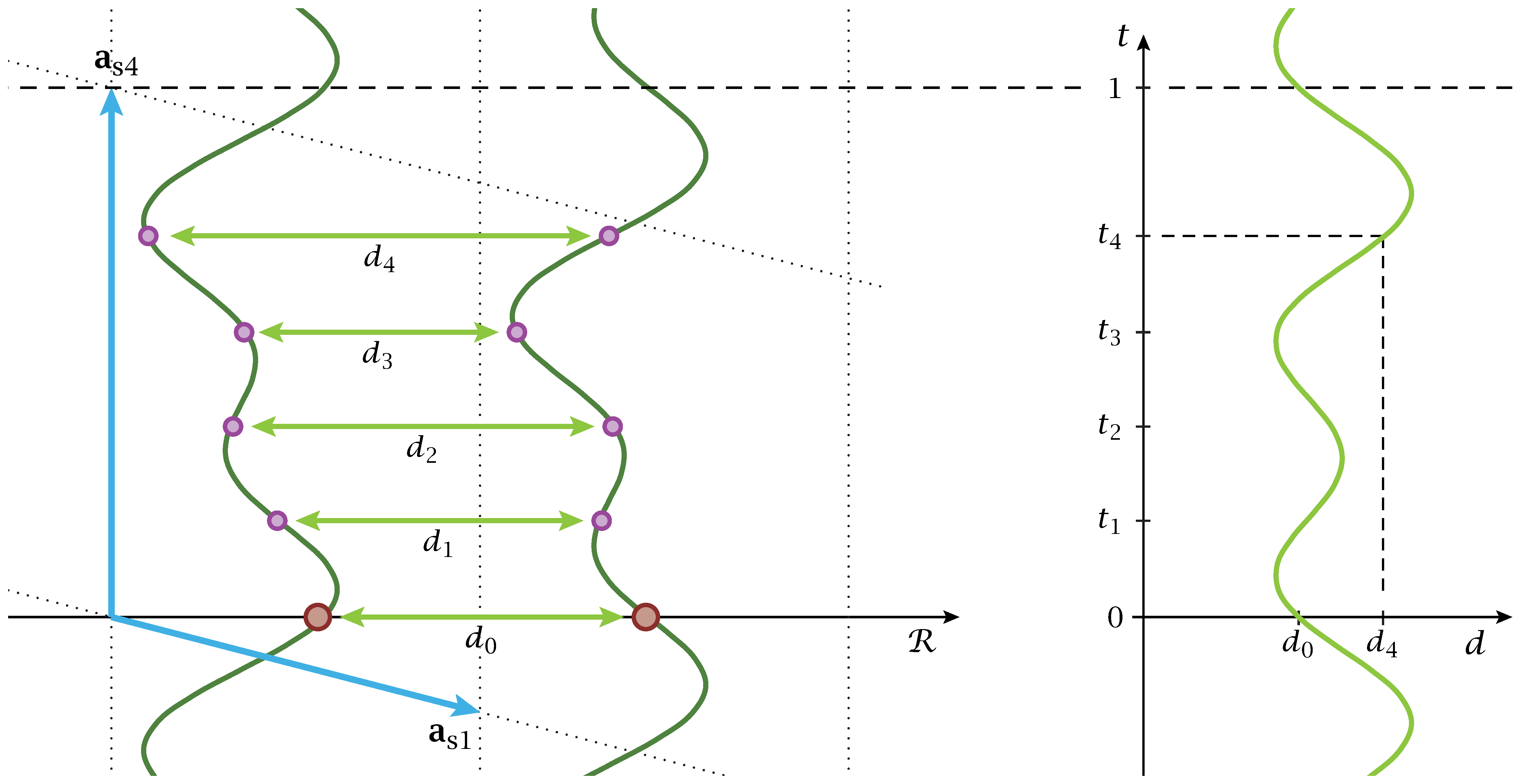
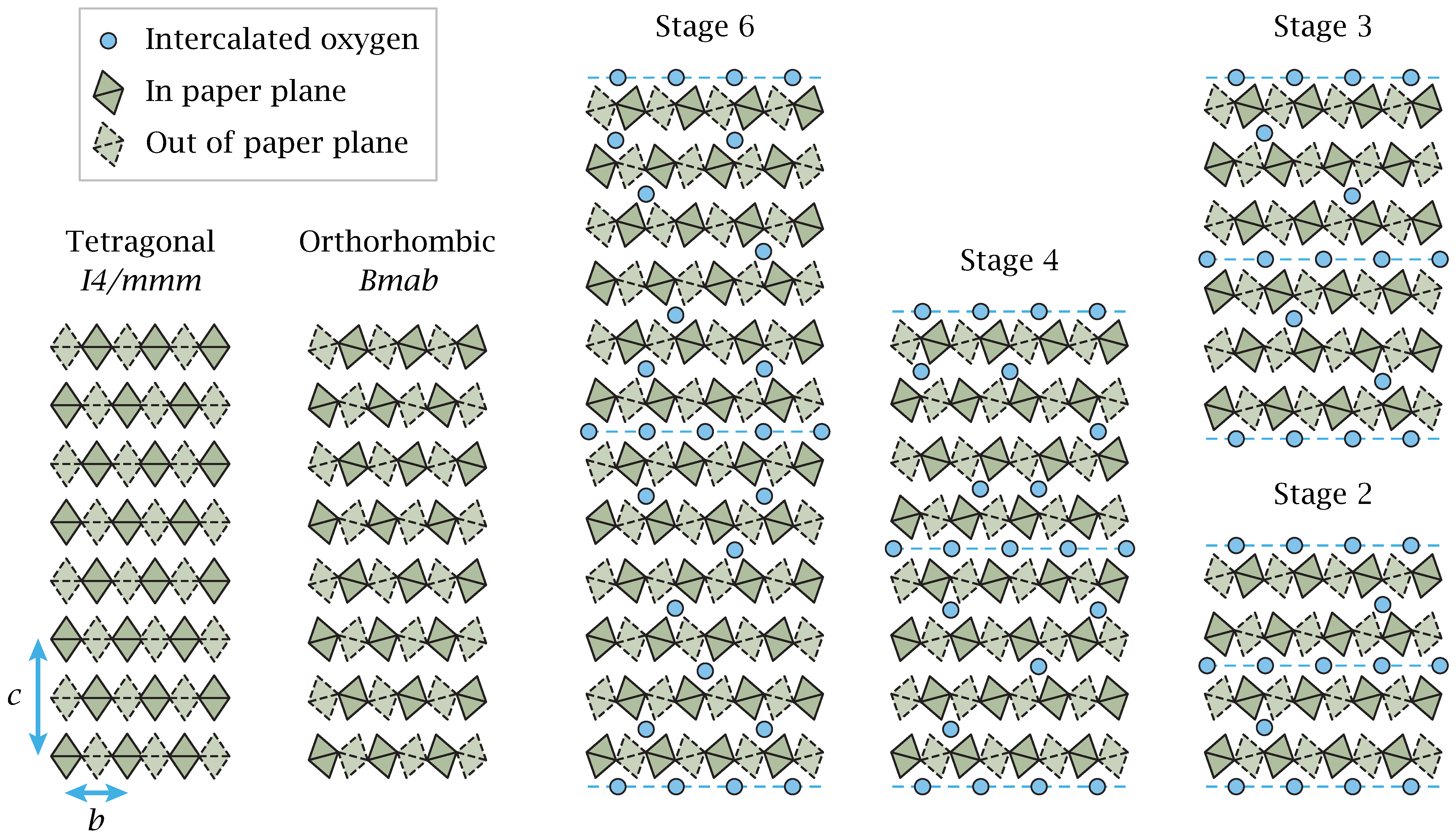
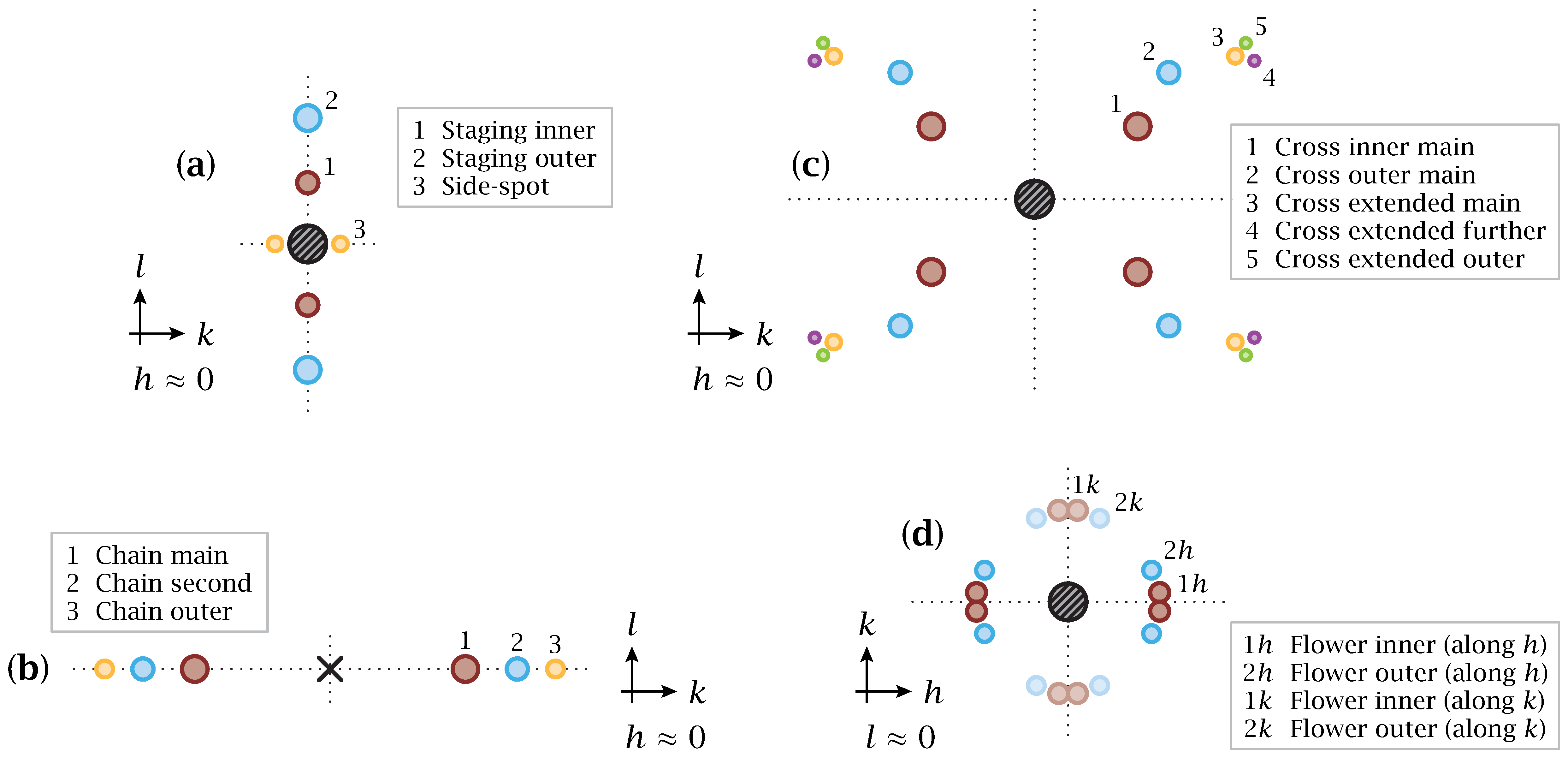
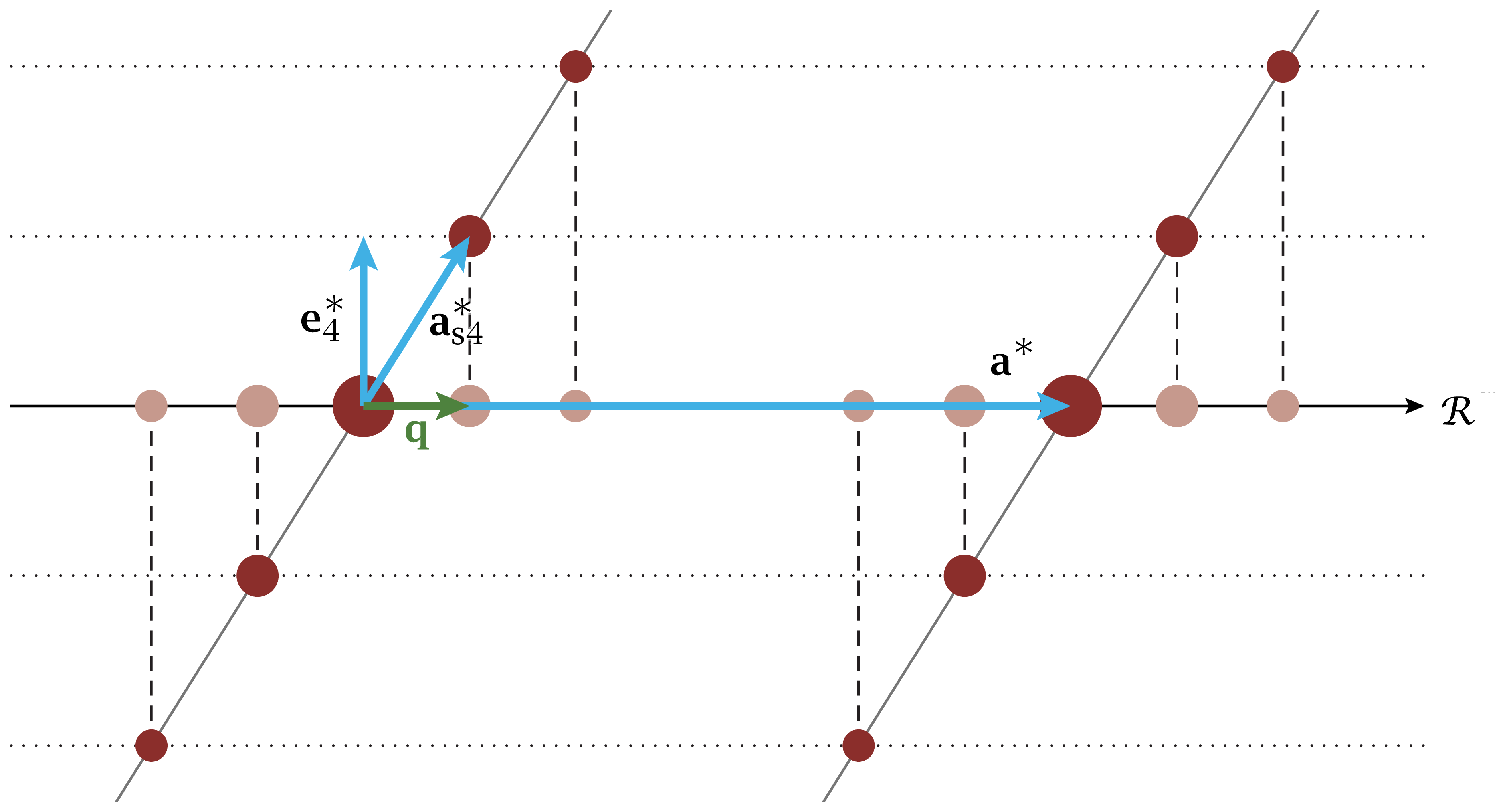
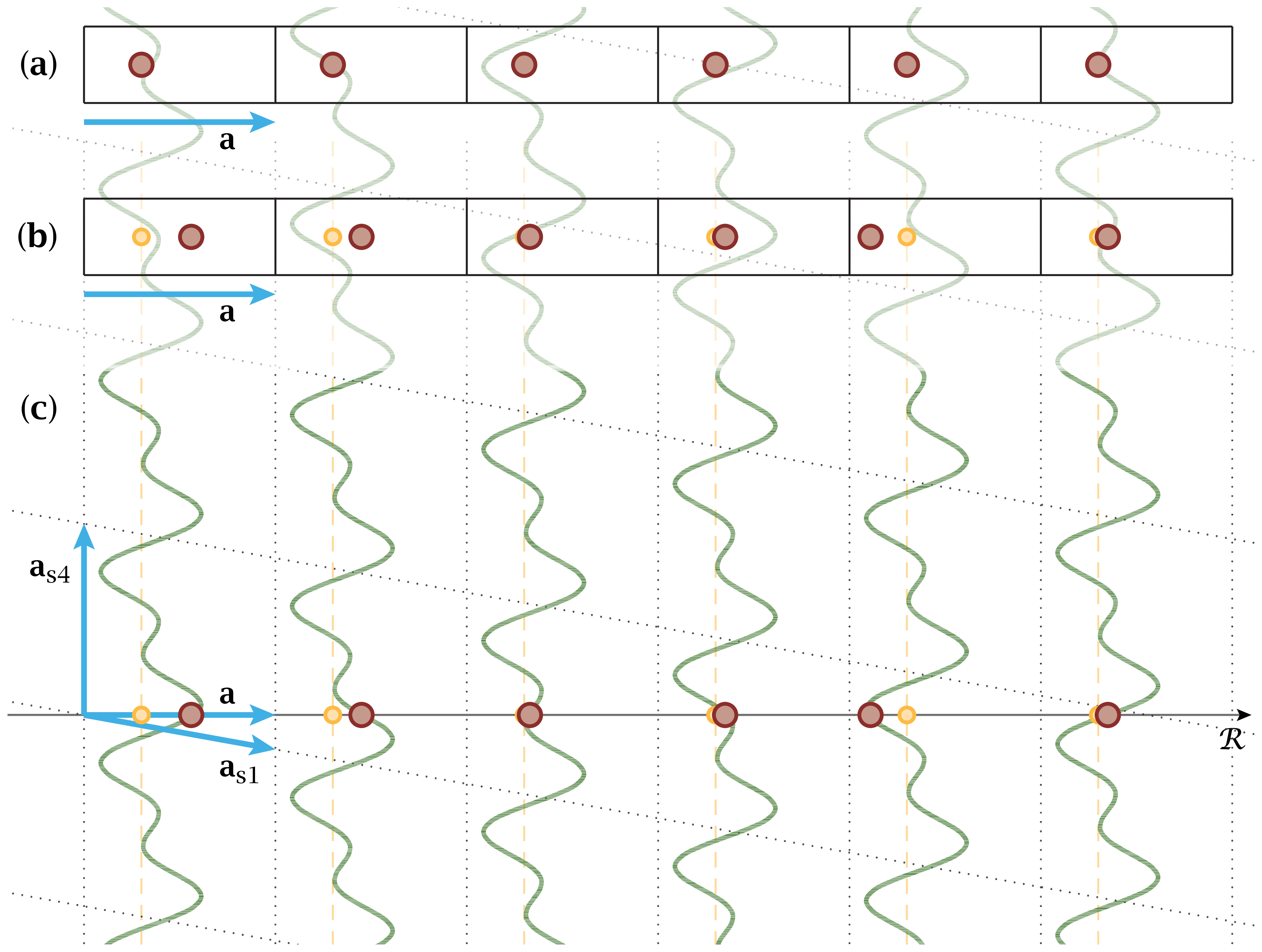
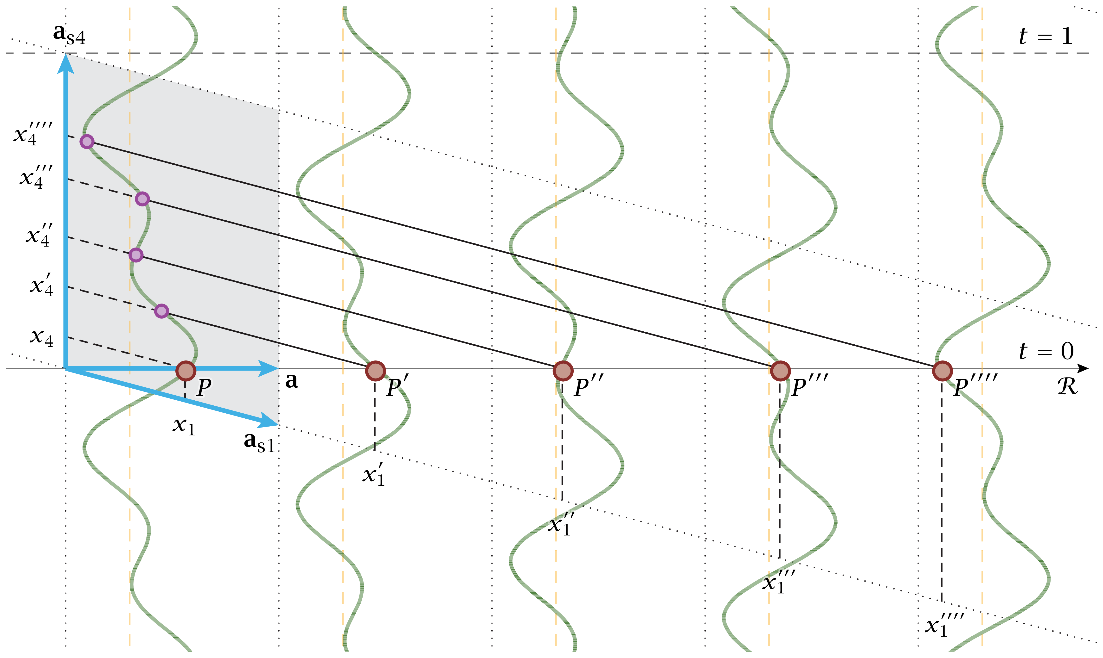
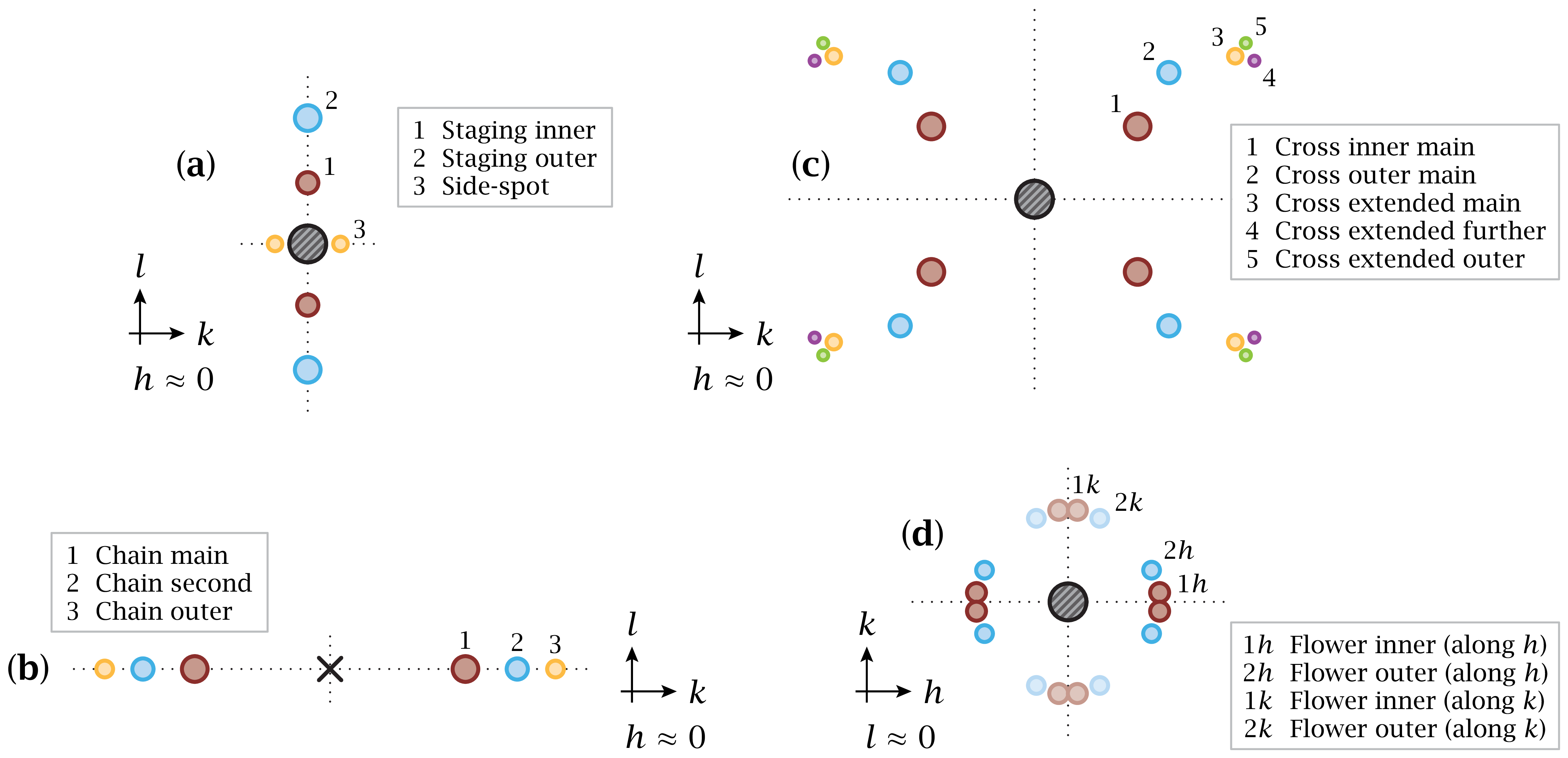
Figur 8.13: Overviews of naming for four of the superstructures discussed for La(2)CuO(4+y). Download links:PNG • αPNG • SVG • PDF. .
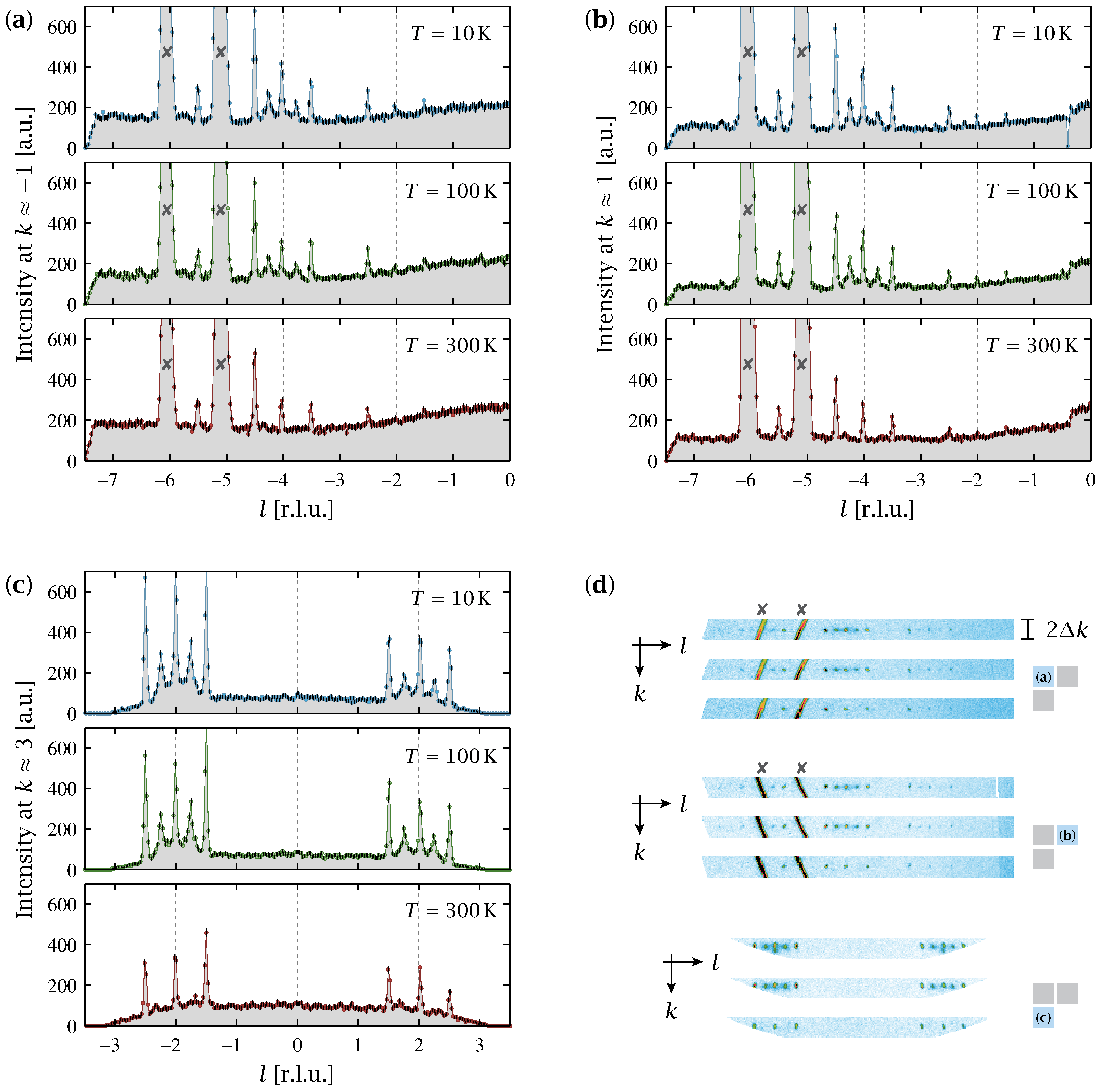
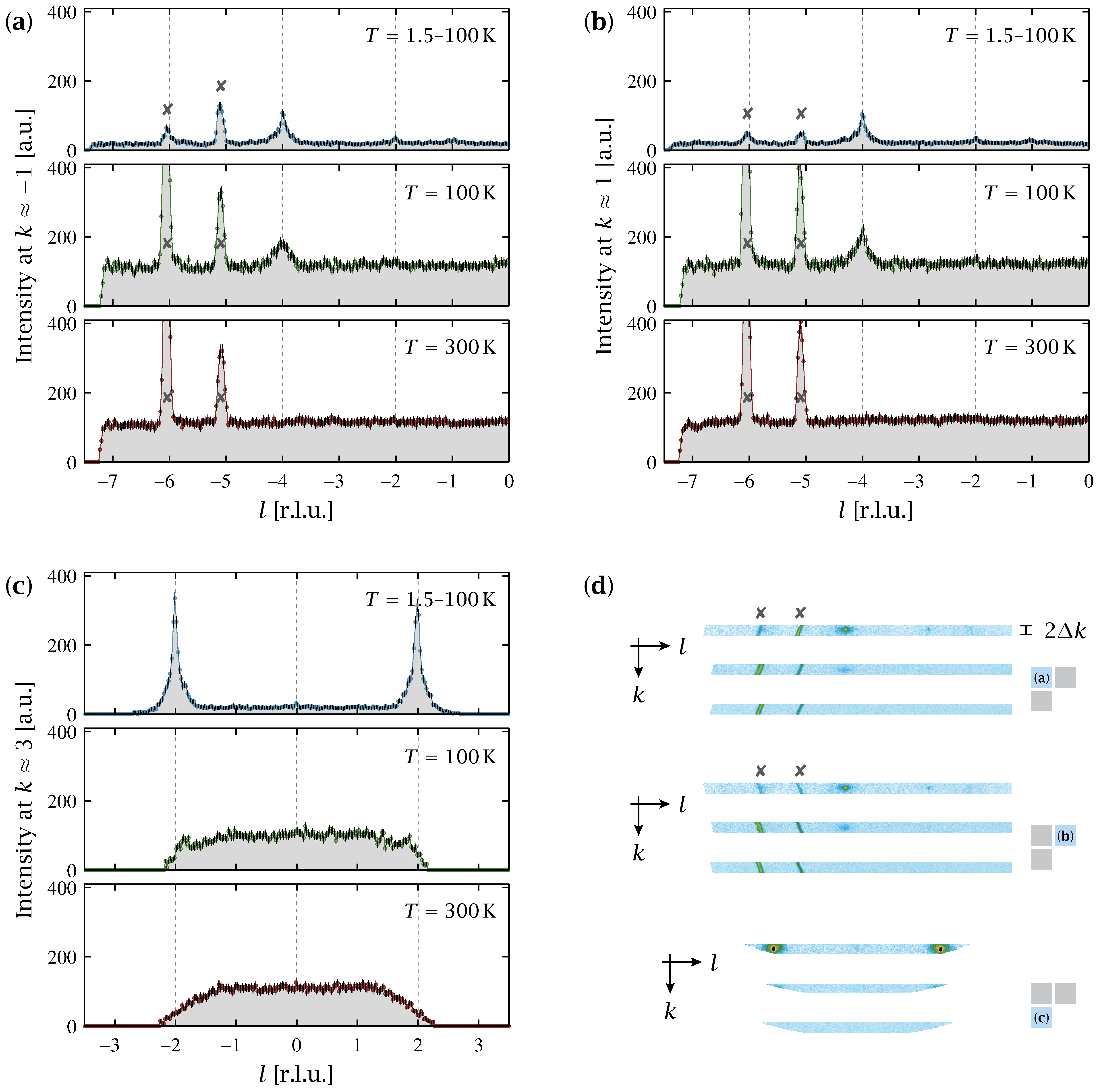
Figur 8.14: Staging - data collapsed along k for the La(2)CuO(4+y) sample. Download links:PNG • SVG • PDF. .
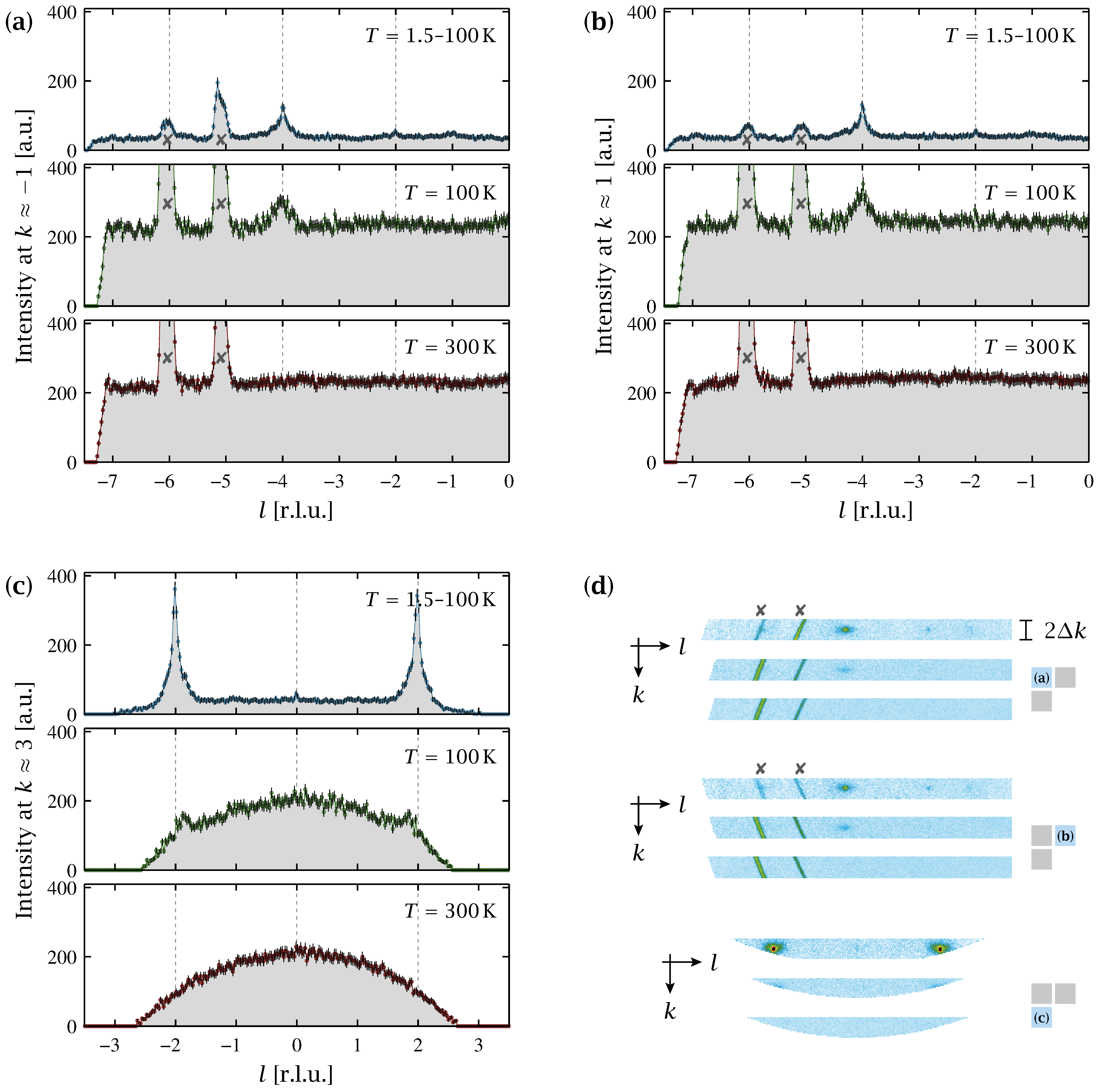
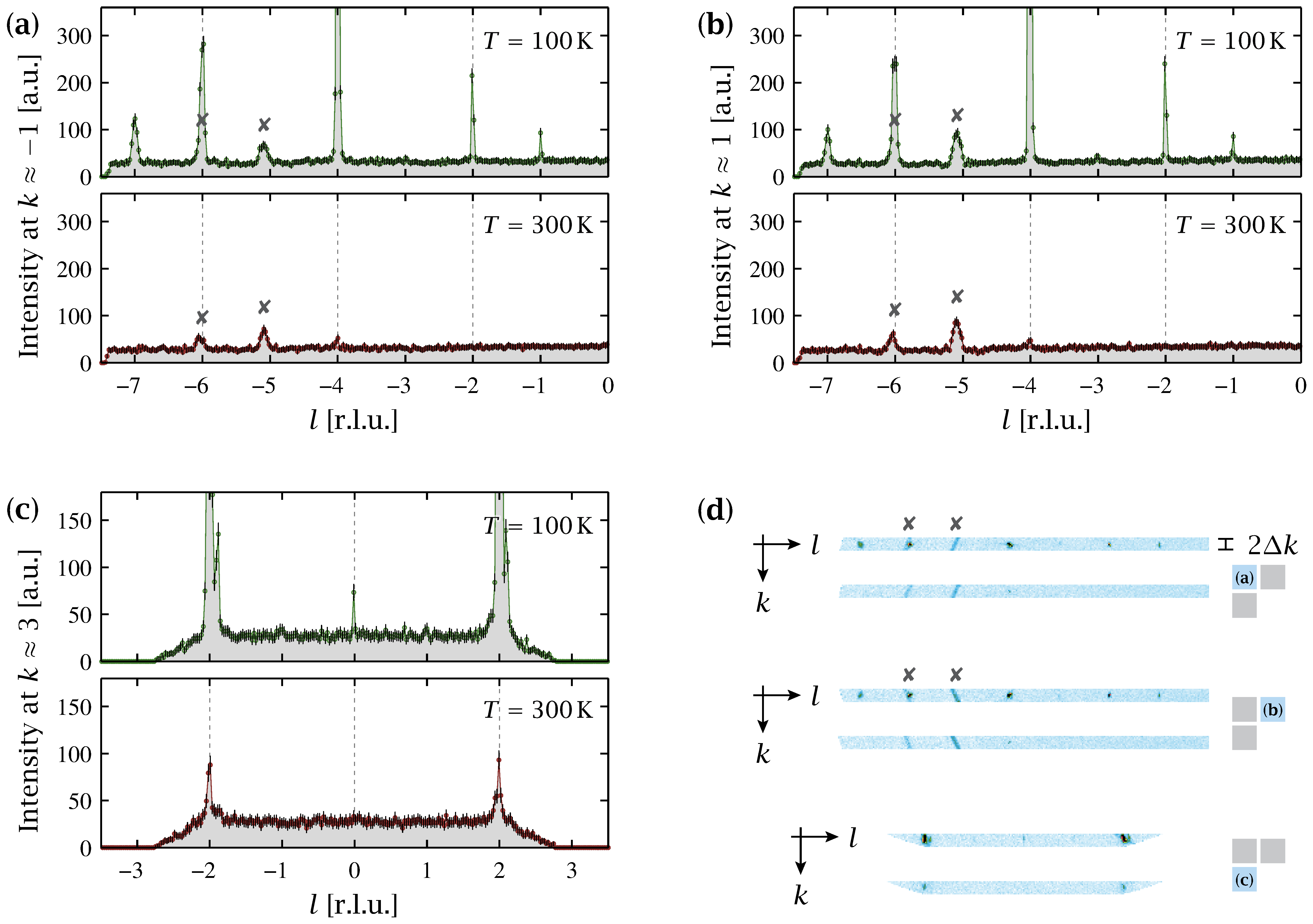
Figur 8.15: Staging - data collapsed along k for the La(1.94)Sr(0.06)CuO(4+y) sample. Download links:PNG • SVG • PDF. .
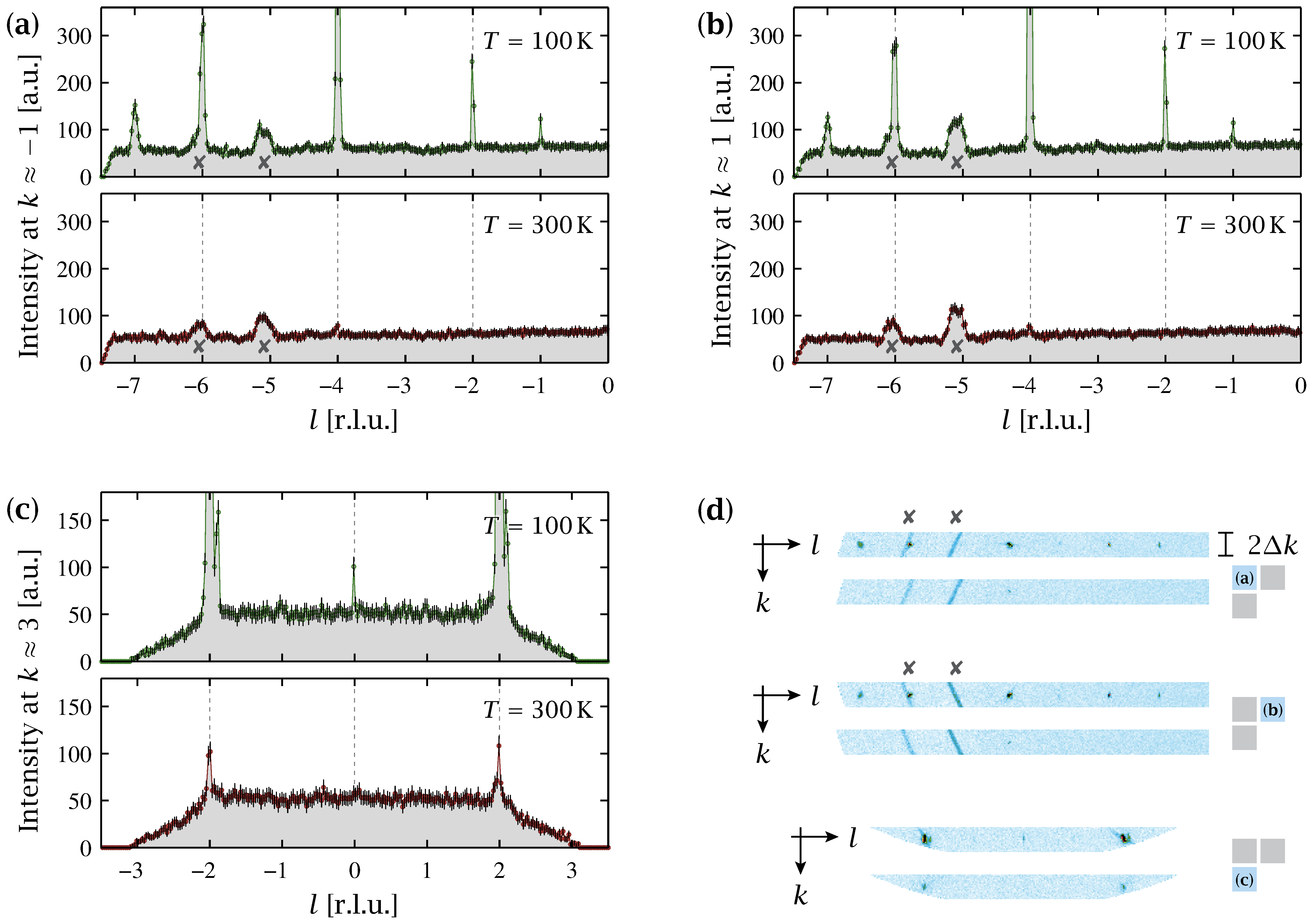
Figur 8.16: Staging - data collapsed along k for the La(1.91)Sr(0.09)CuO(4+y) sample. Download links:PNG • SVG • PDF. .
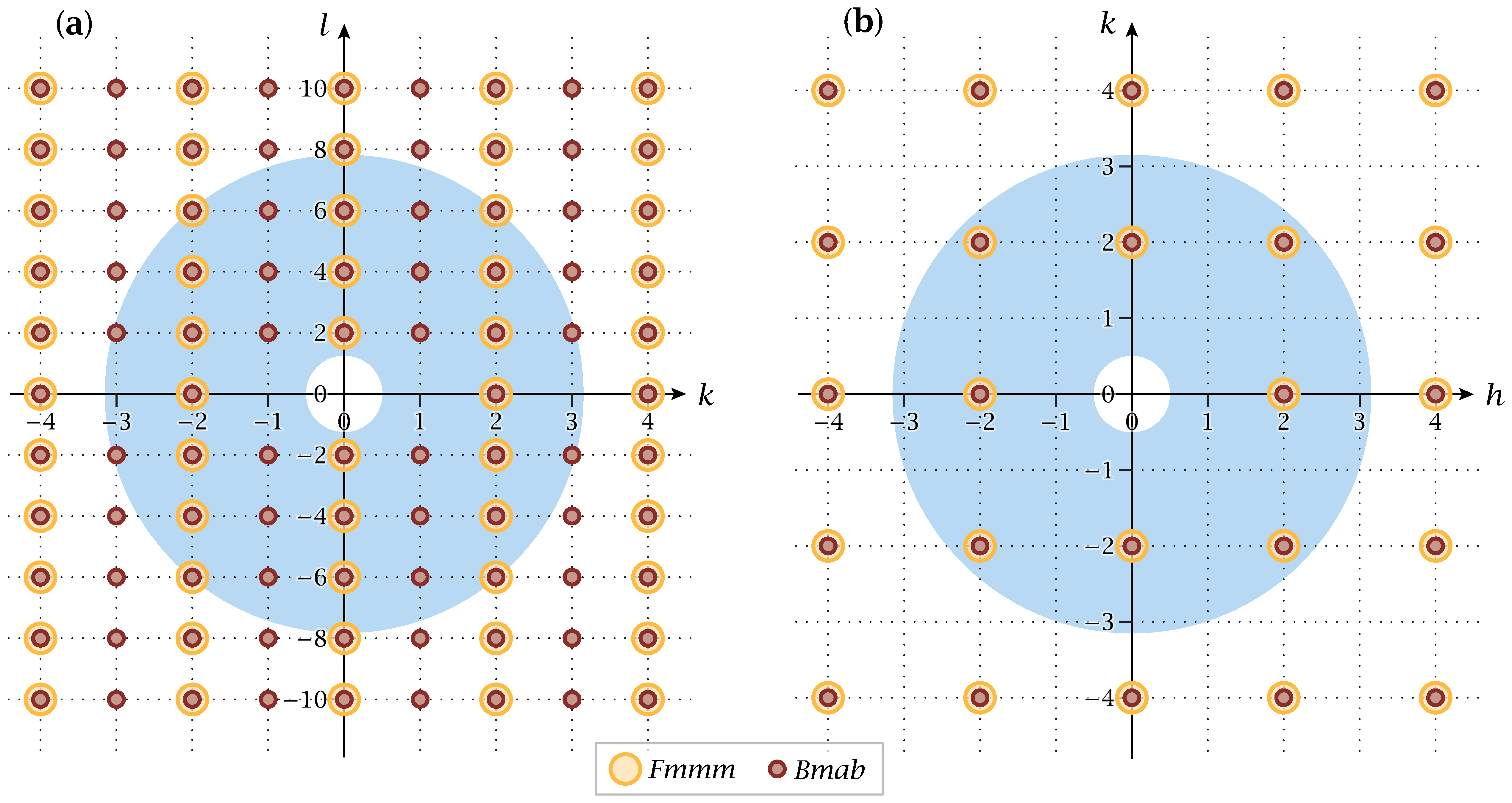
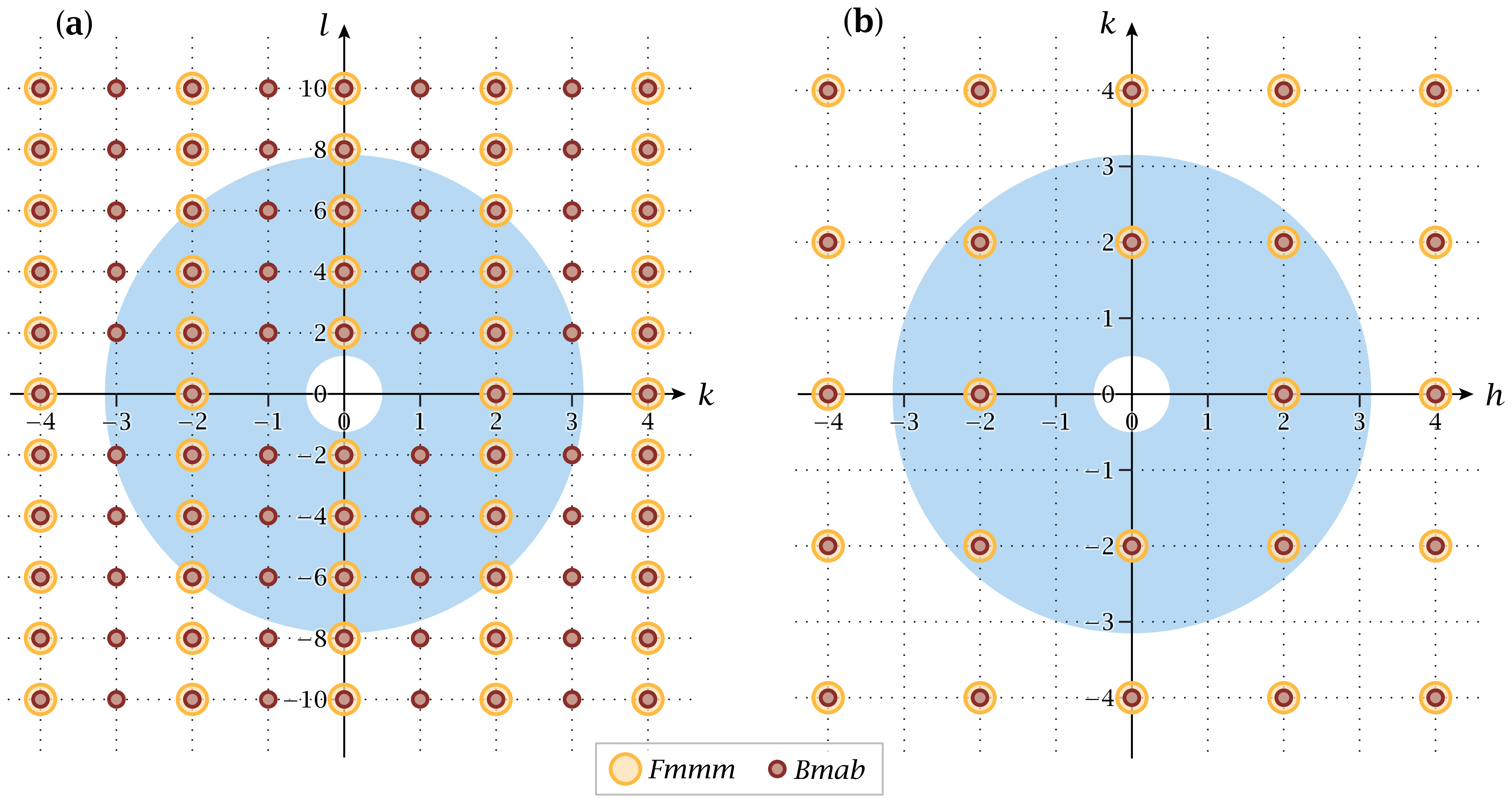
Figur 8.17: Allowed reflections in the (0kl) and (hk0) planes. Download links:PNG • αPNG • SVG • PDF. .
Figur 8.18: Chain data - for the La(2)CuO(4+y) sample collapsed along l. Download links:PNG • SVG • PDF. .
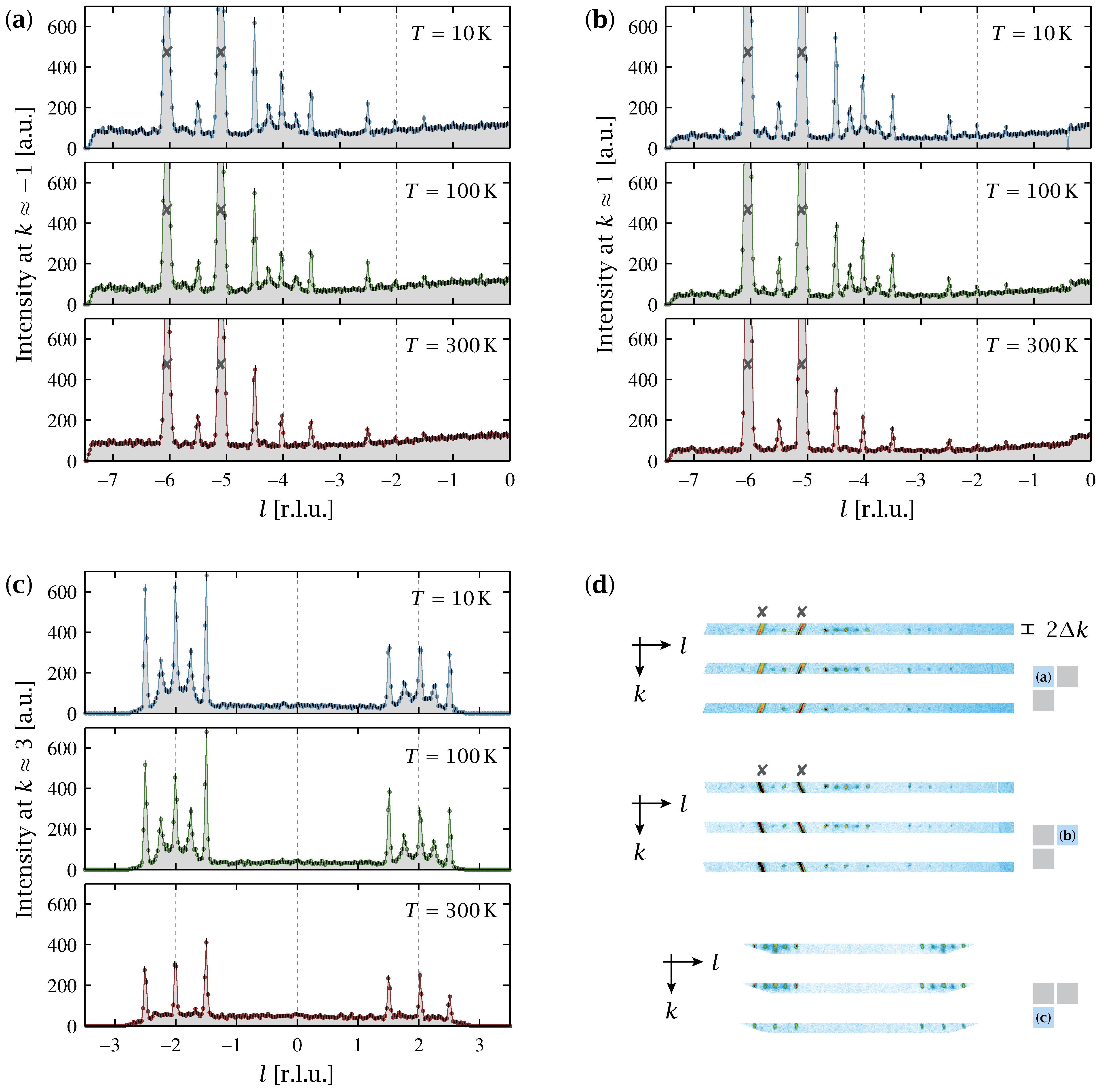
Figur 8.19: Crosses - example of collapsed data for La(2)CuO(4+y) at T = 10 K and 300 K. Download links:PNG • SVG • PDF. .
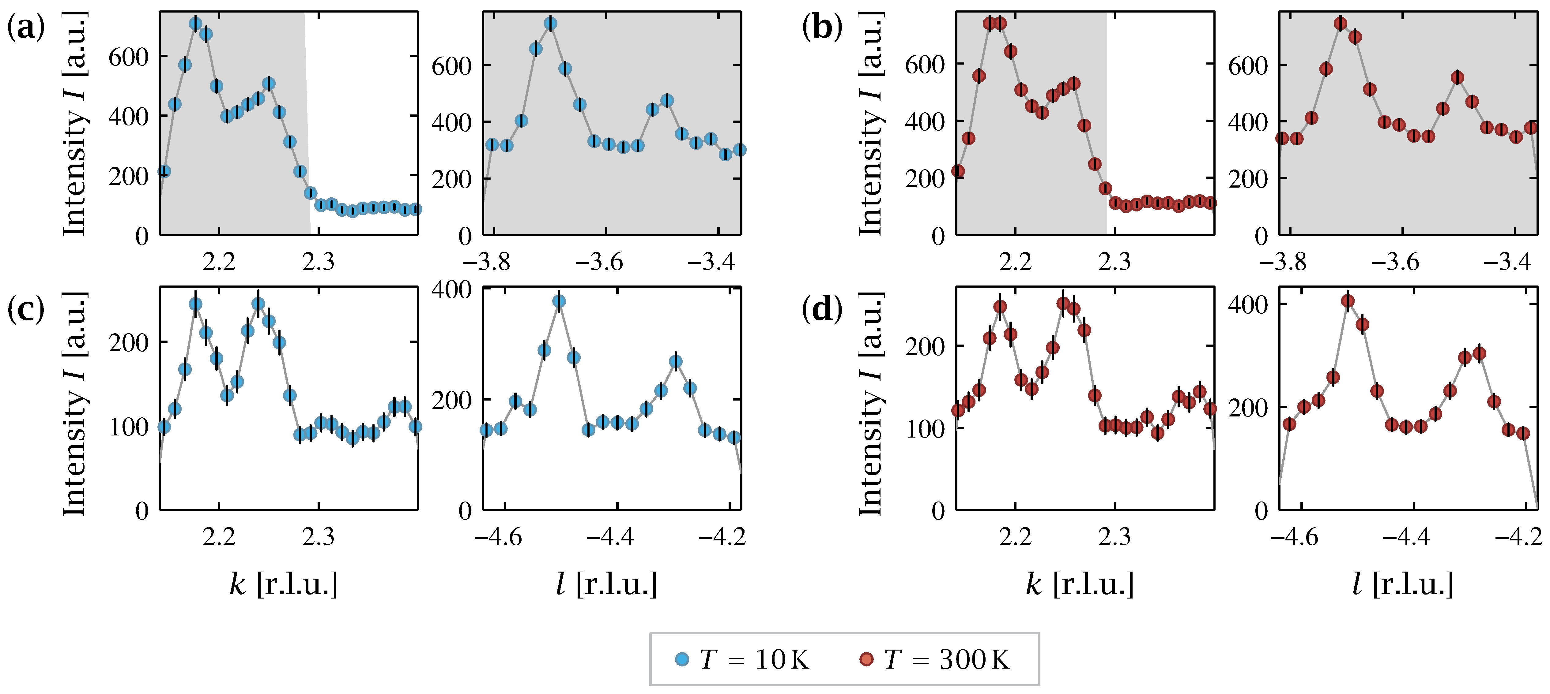
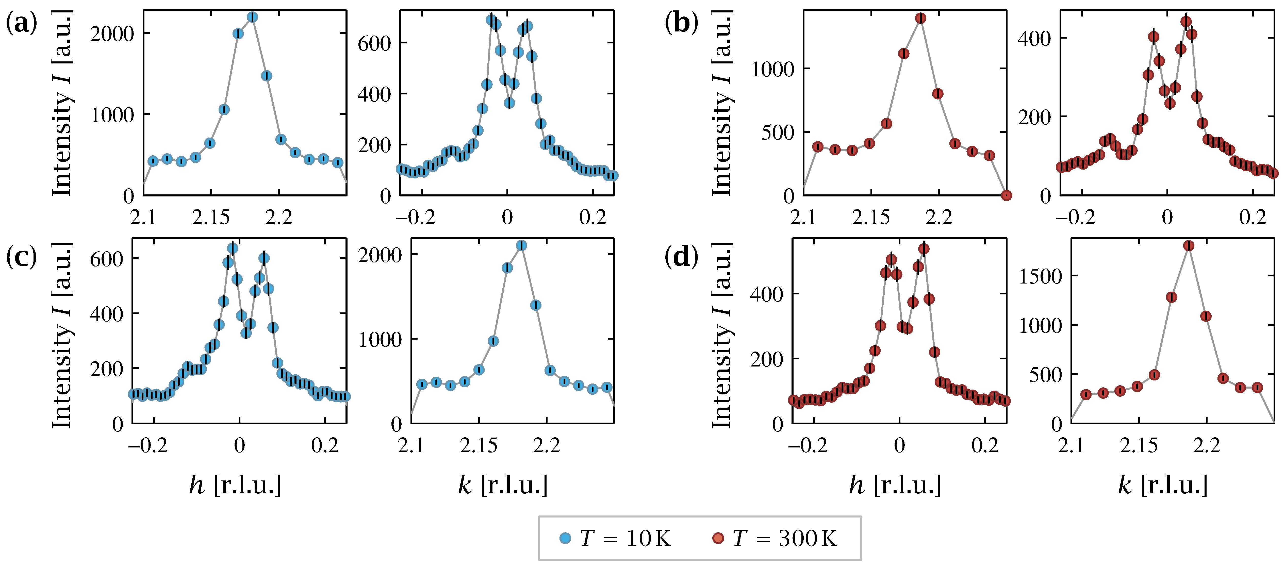
Figur 8.20: Flowers - example of collapsed data for La(2)CuO(4+y) at T = 10 K and 300 K. Download links:PNG • SVG • PDF. .
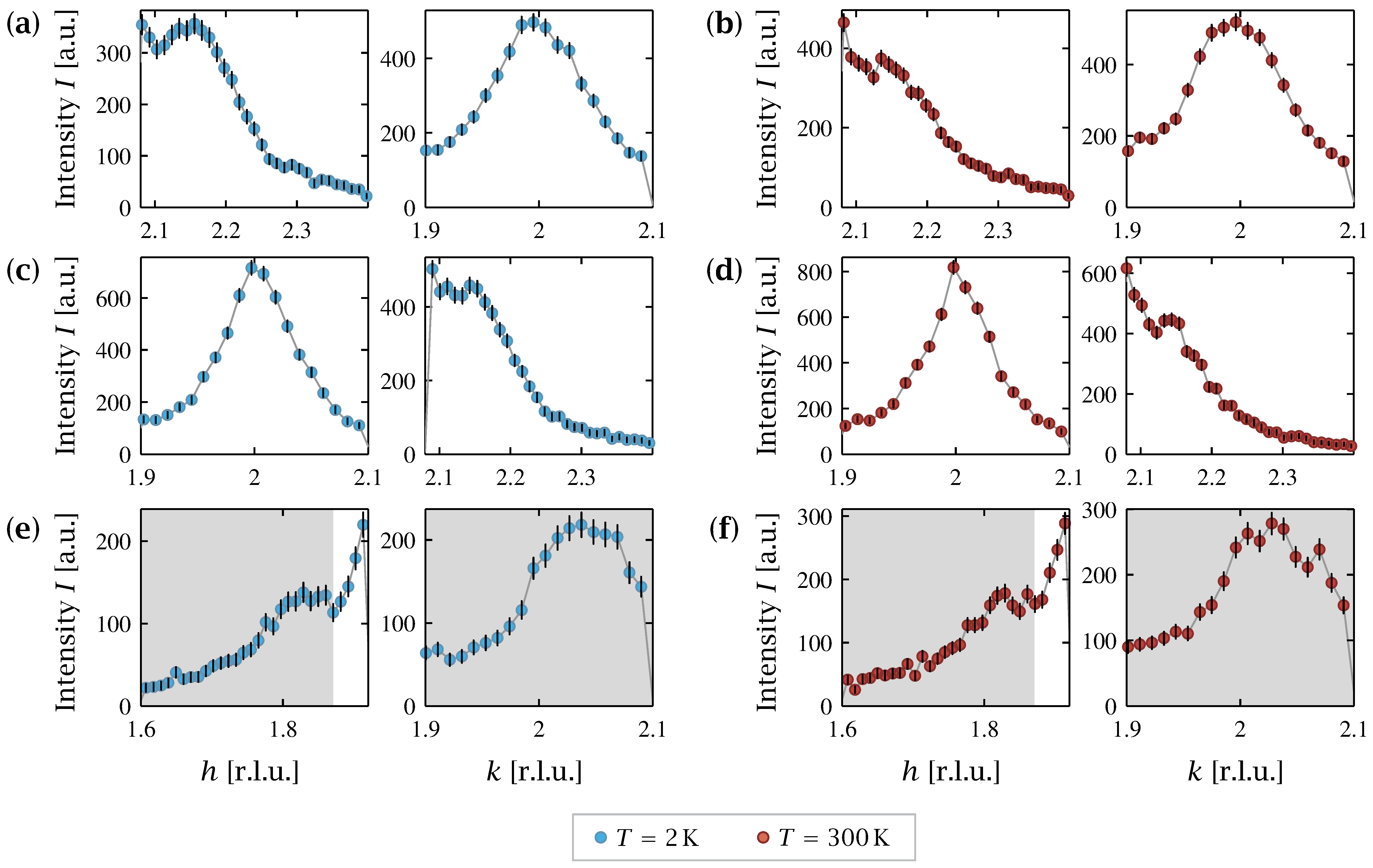
Figur 8.21: Flowers - example of collapsed data for La(1.94)Sr(0.06)CuO(4+y) at T = 2 K and 300 K. Download links:PNG • SVG • PDF. .
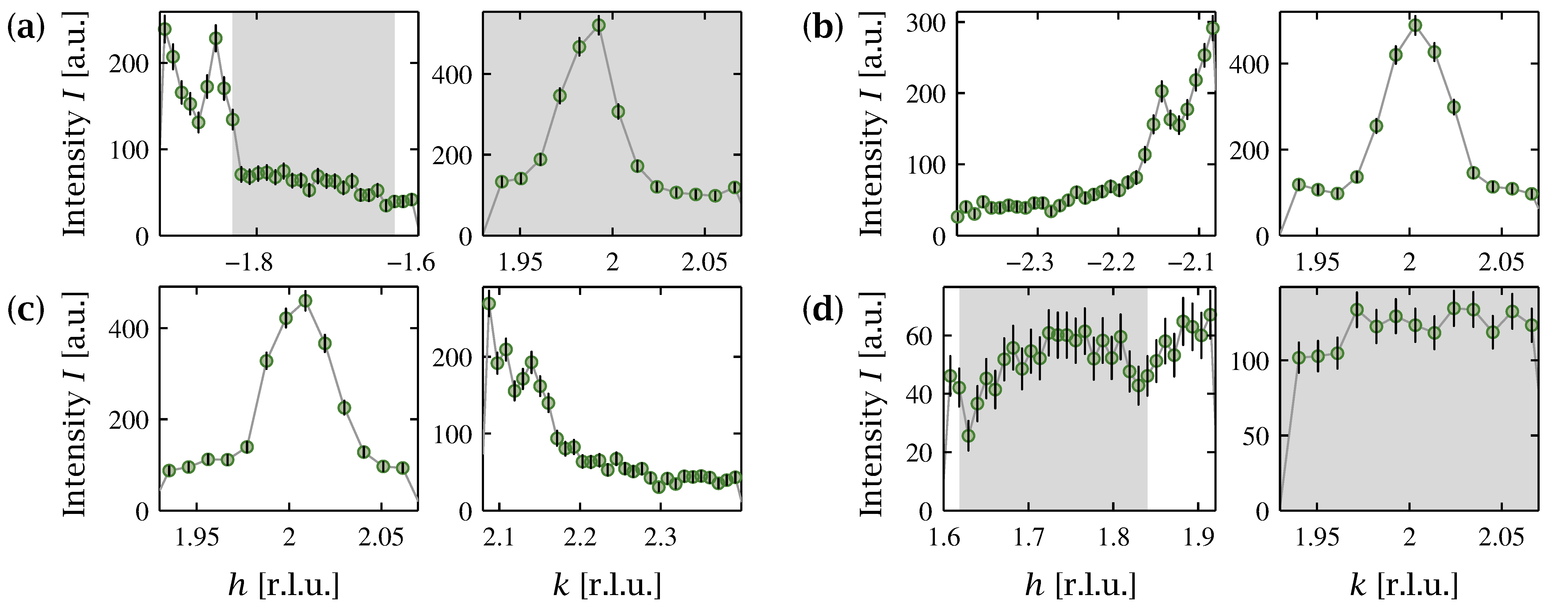
Figur 8.22: Flowers - example of collapsed data for La(1.91)Sr(0.09)CuO(4+y) at T = 100 K. Download links:PNG • SVG • PDF. .
Figur 8.23: Comparing two different La(2)CuO(4+y) sample (0kl) planes. Download links:PNG • SVG • PDF. .
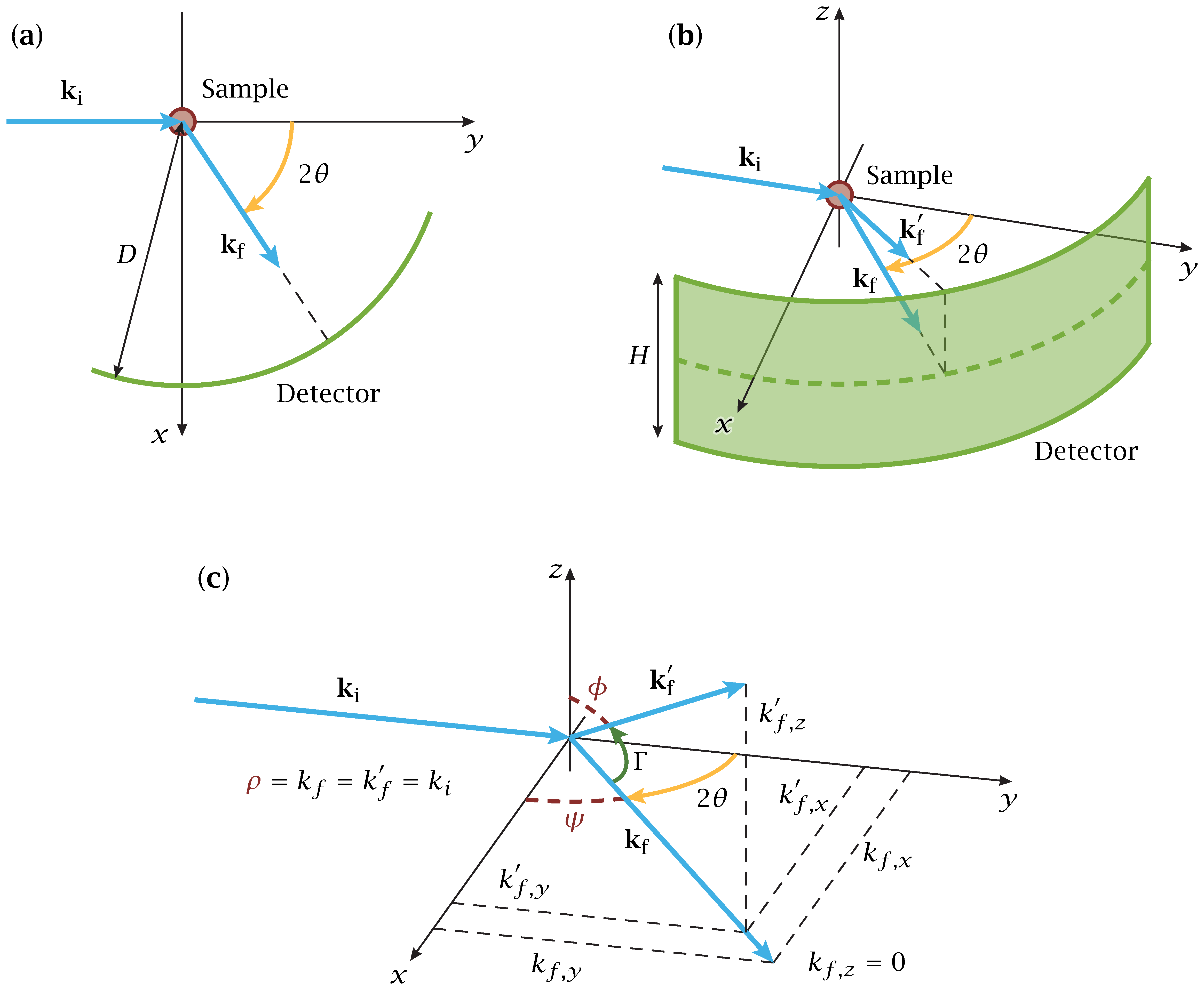
Figur A.5: Coordinate system used for the calculation with DMC detector height. Download links:PNG • αPNG • SVG • PDF. .
SXD-illustrationer og dataplots (kapitel 9)
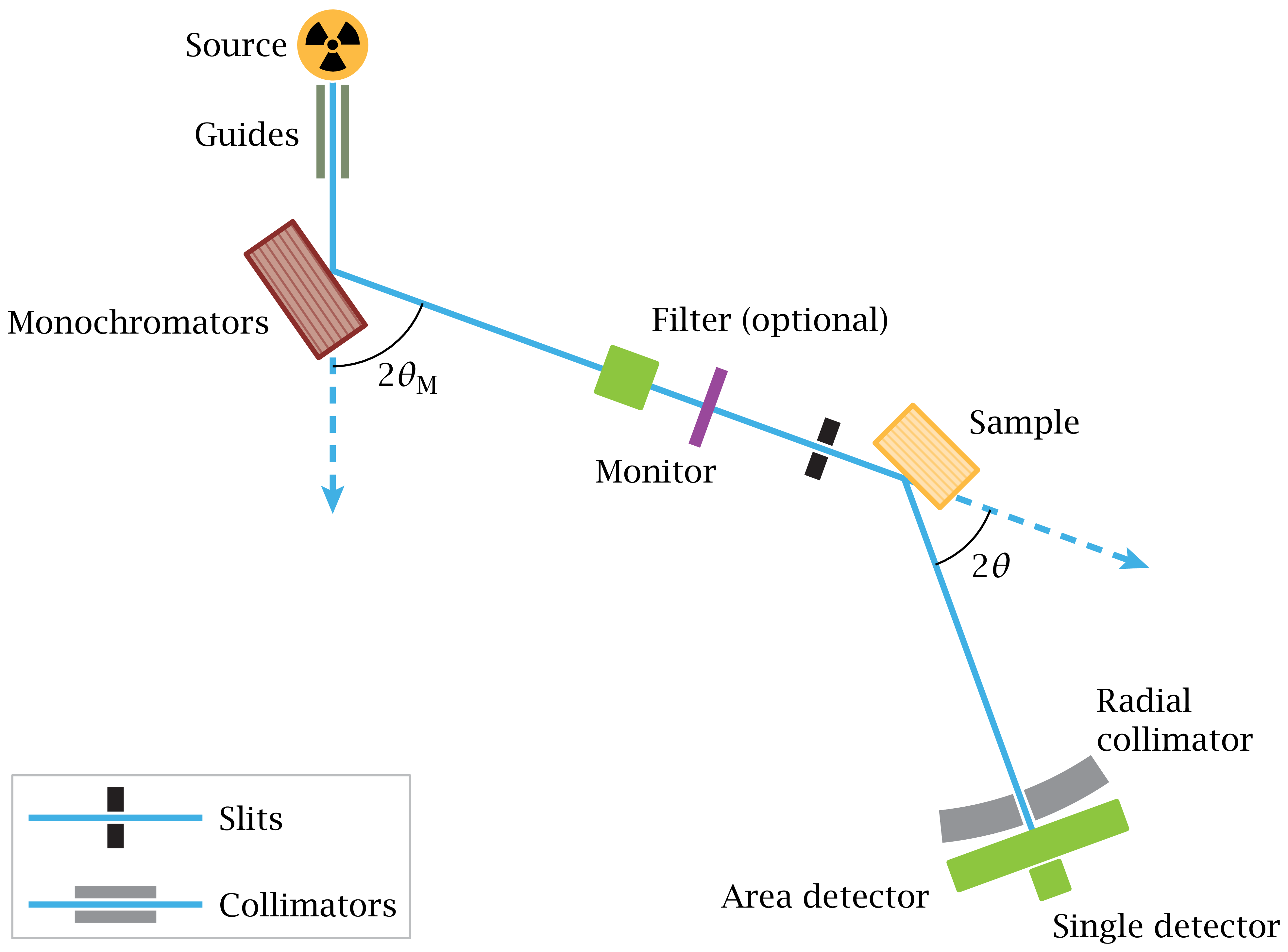
Figur 9.1: Overview sketch of the SXD instrument. Download links:PNG • αPNG • SVG • PDF. .
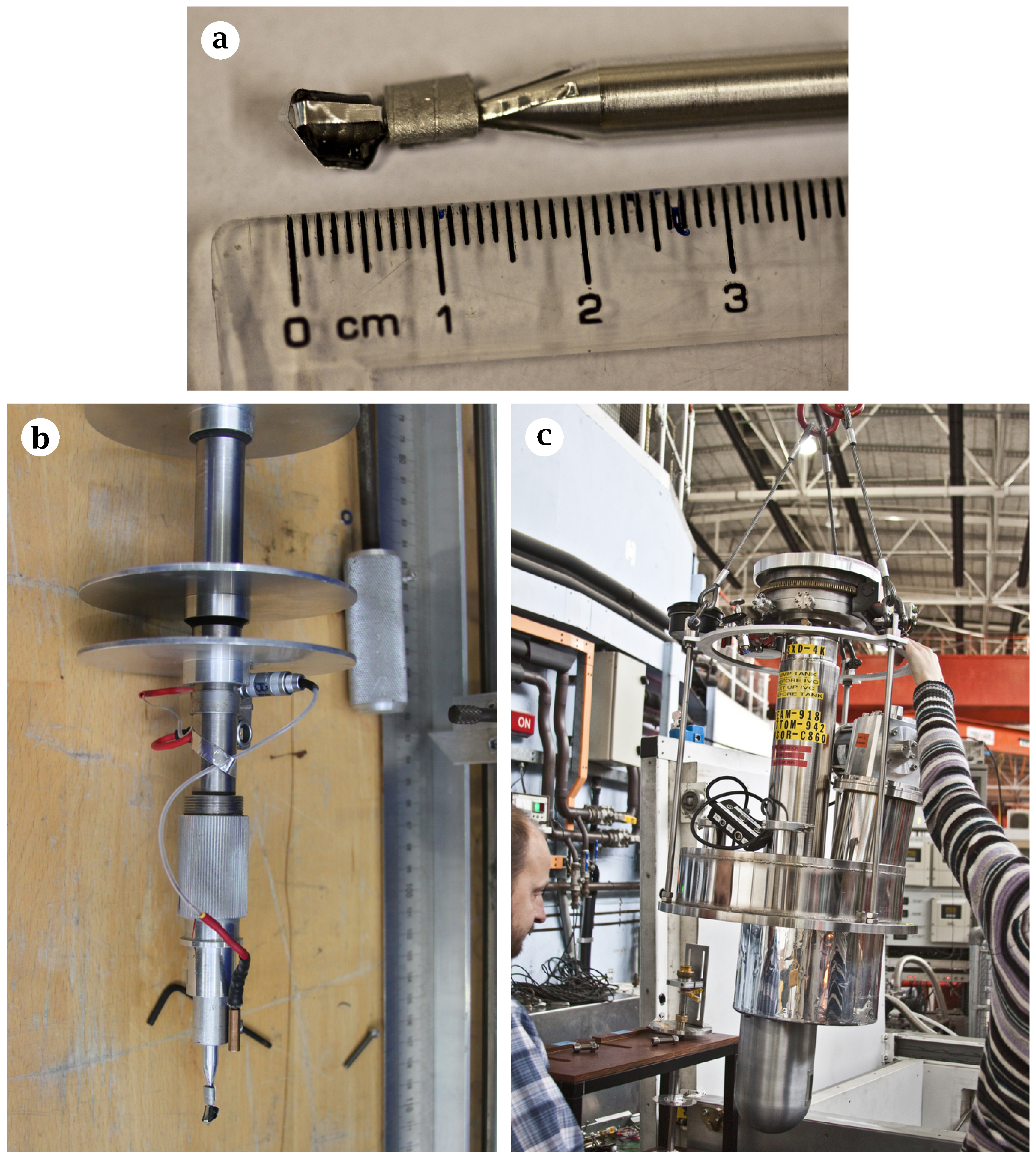
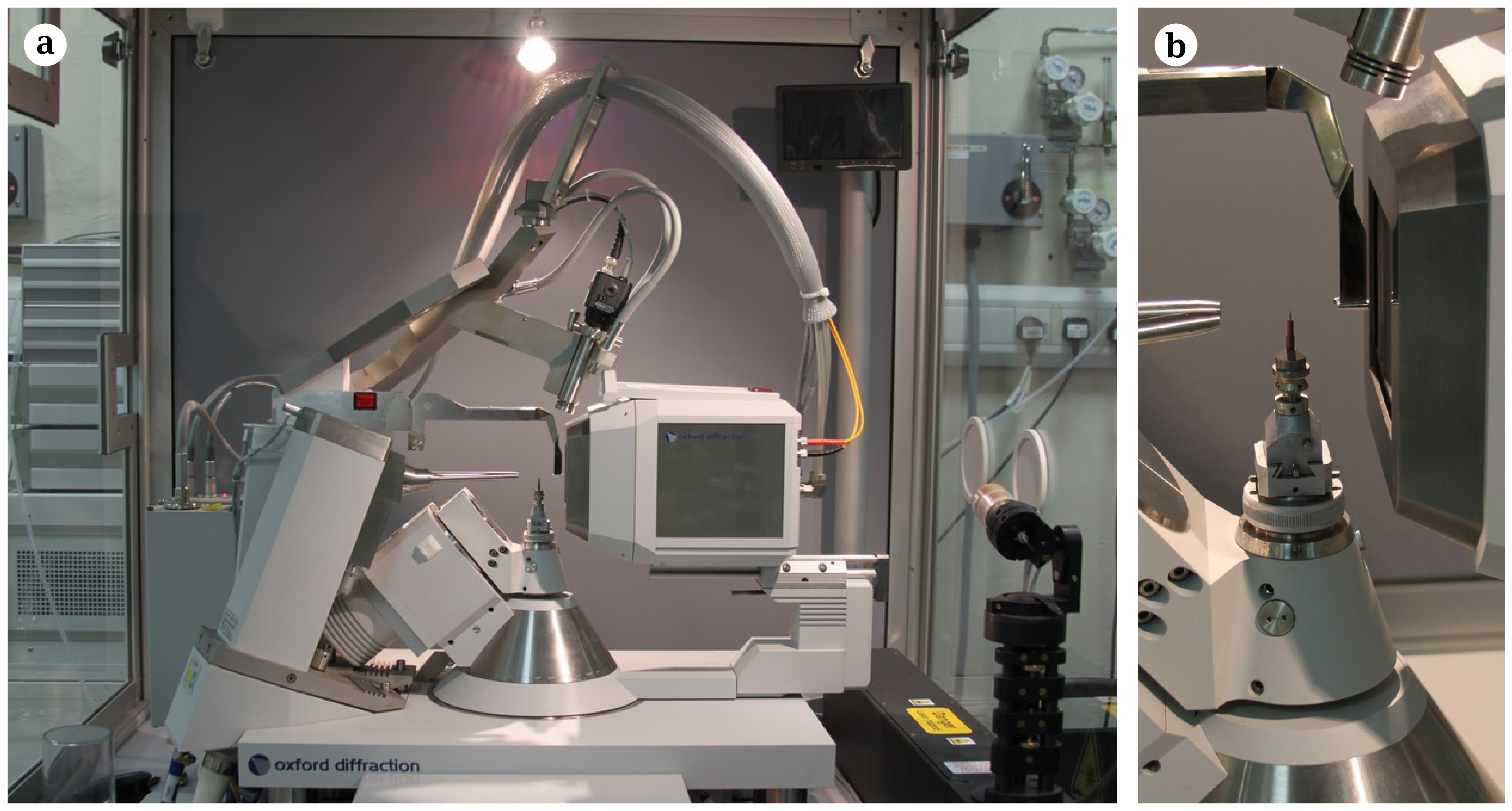
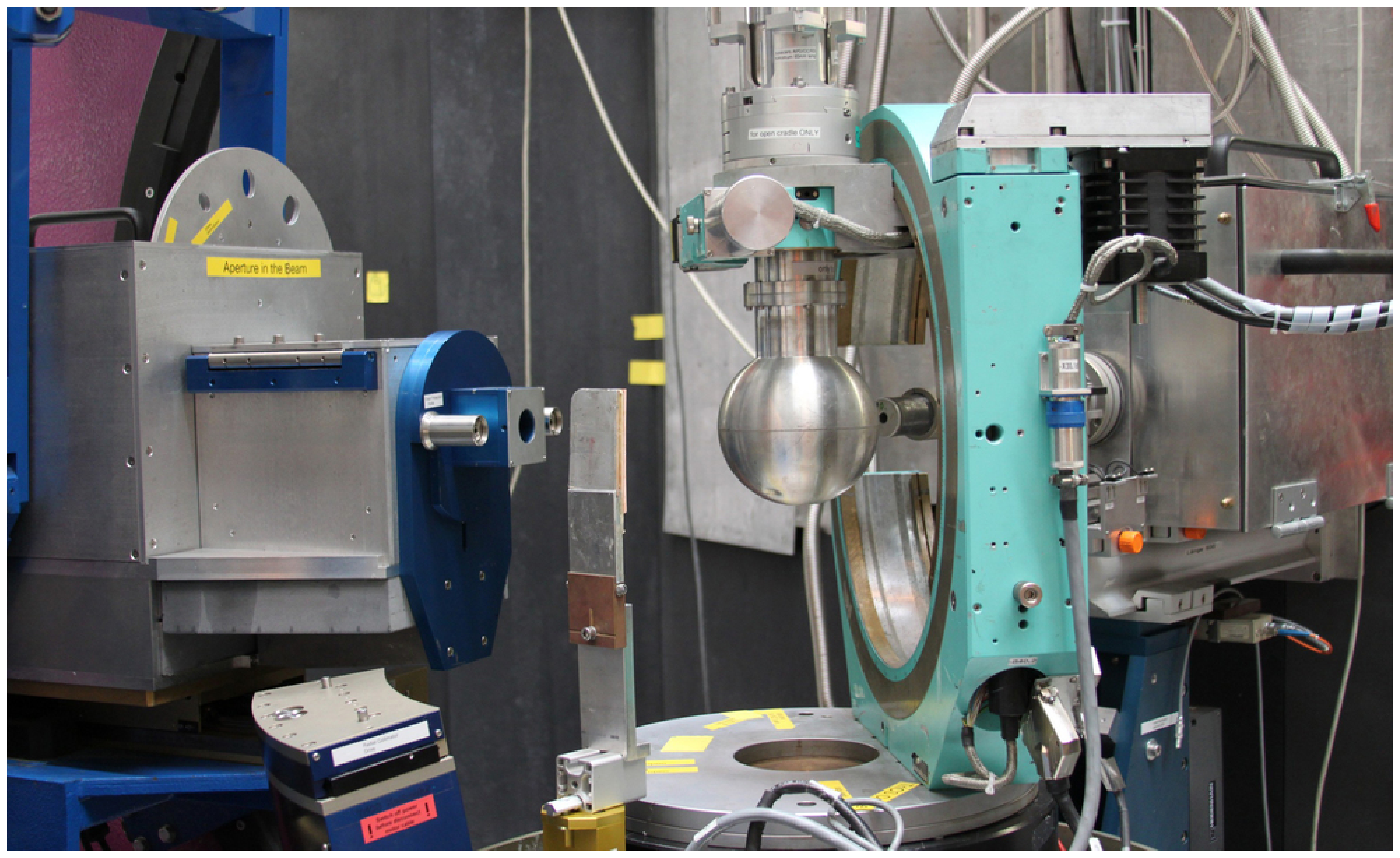
Figur 9.2: Photos of the SXD instrument. Download links:PNG • SVG • PDF. .
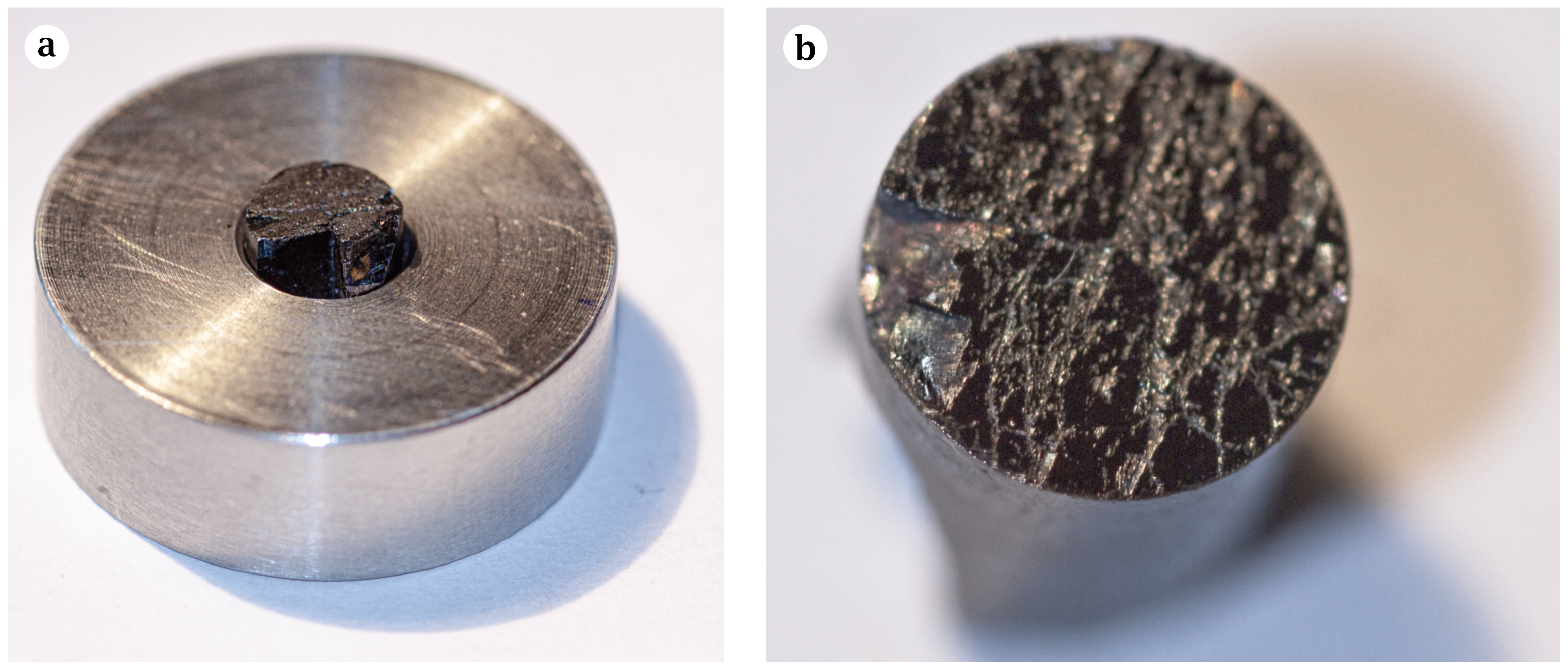
Figur 9.3: The La(2)CuO(4+y) sample measured on SXD. Download links:PNG • αPNG • SVG • PDF. .
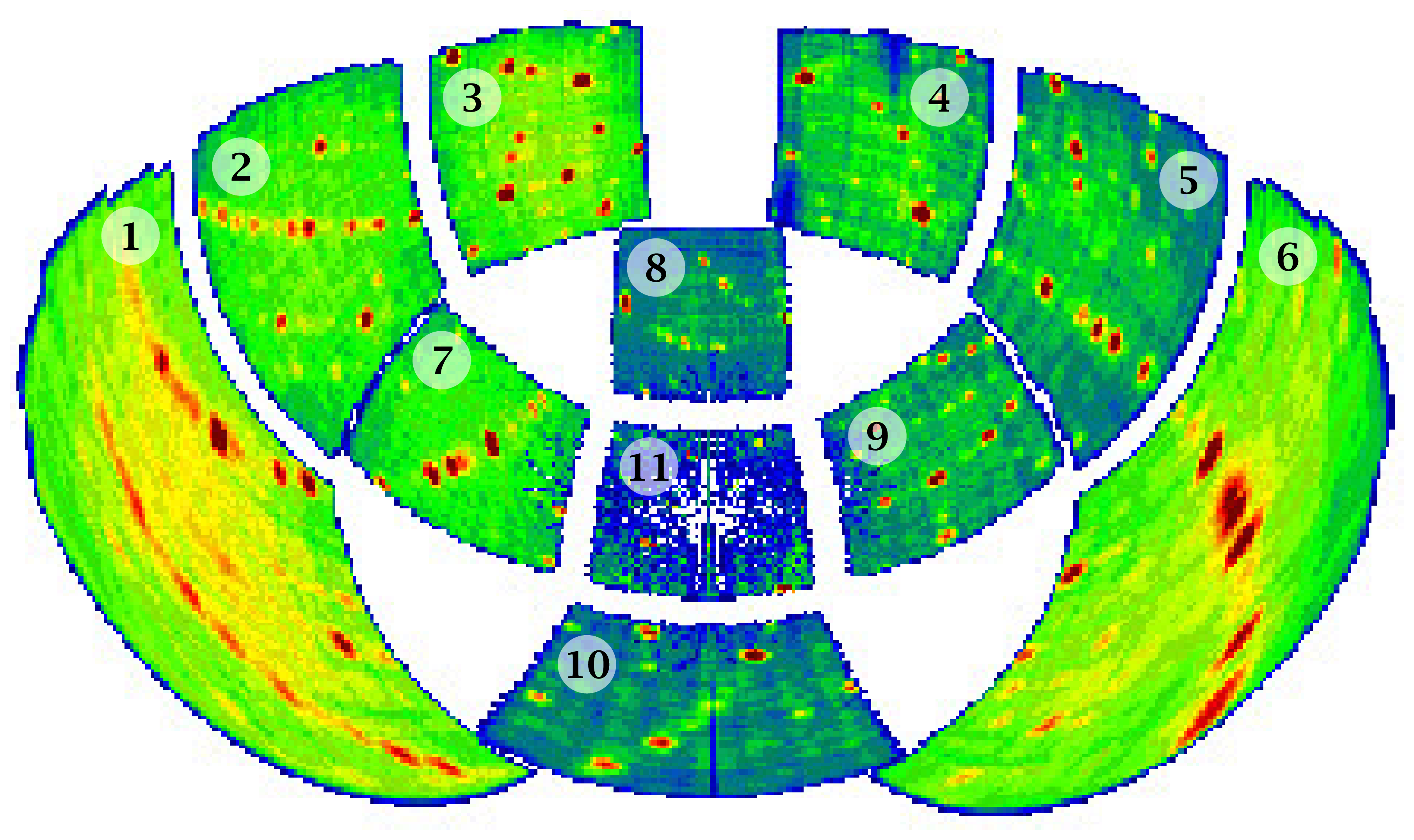
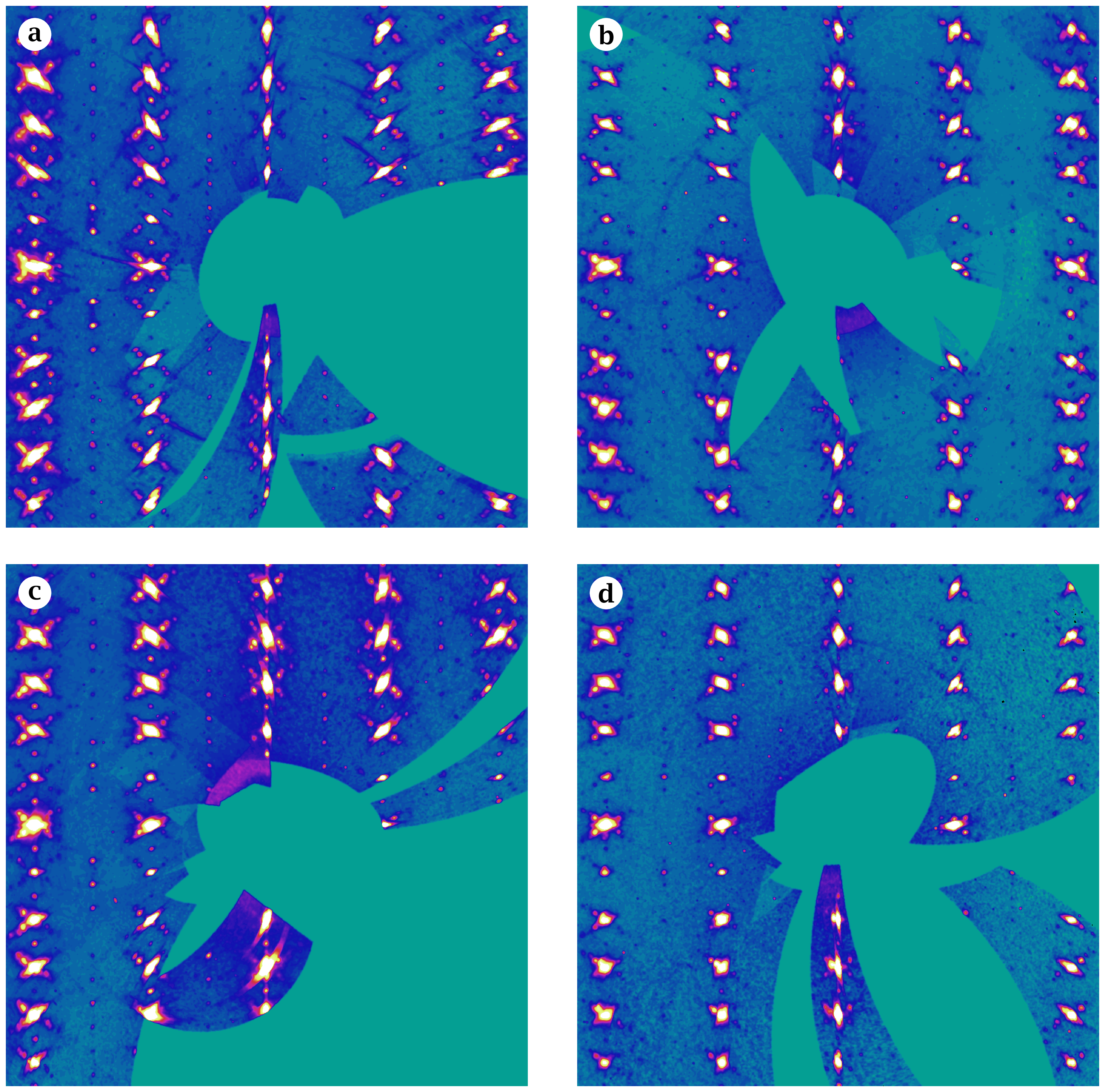
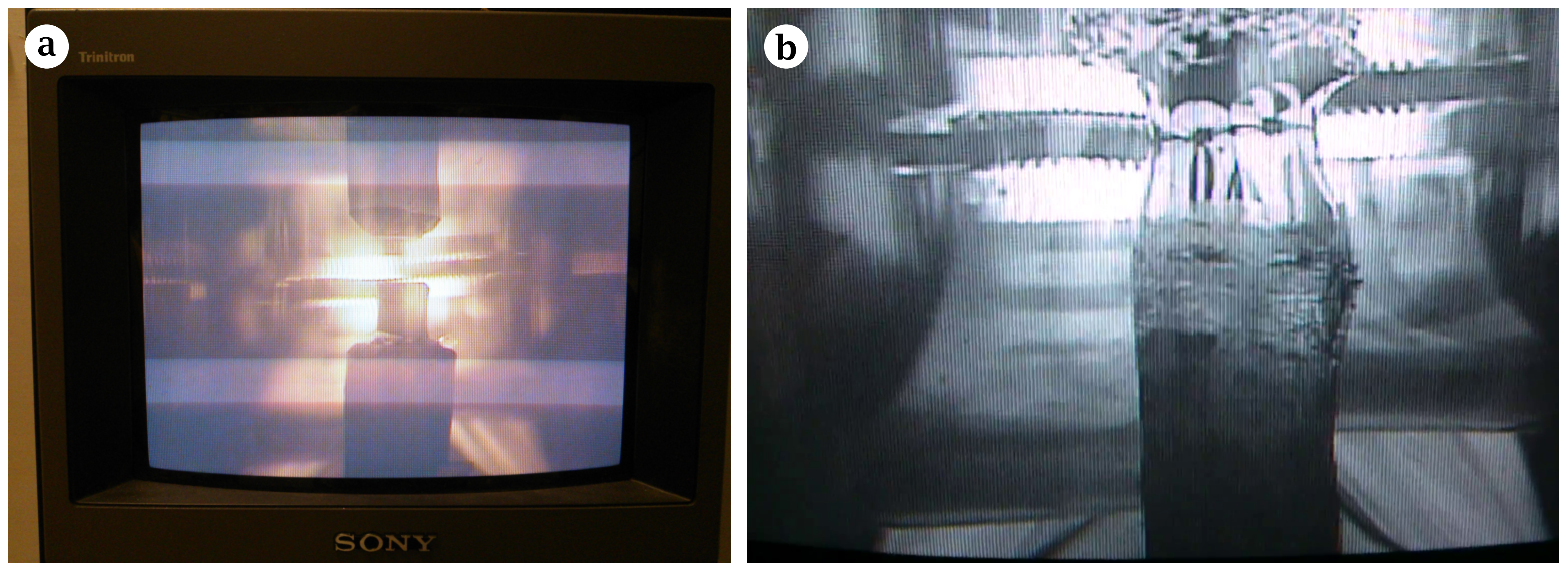
Figur 9.4: Example of a Laue view from the SXD instrument. Download links:PNG • SVG • PDF. .
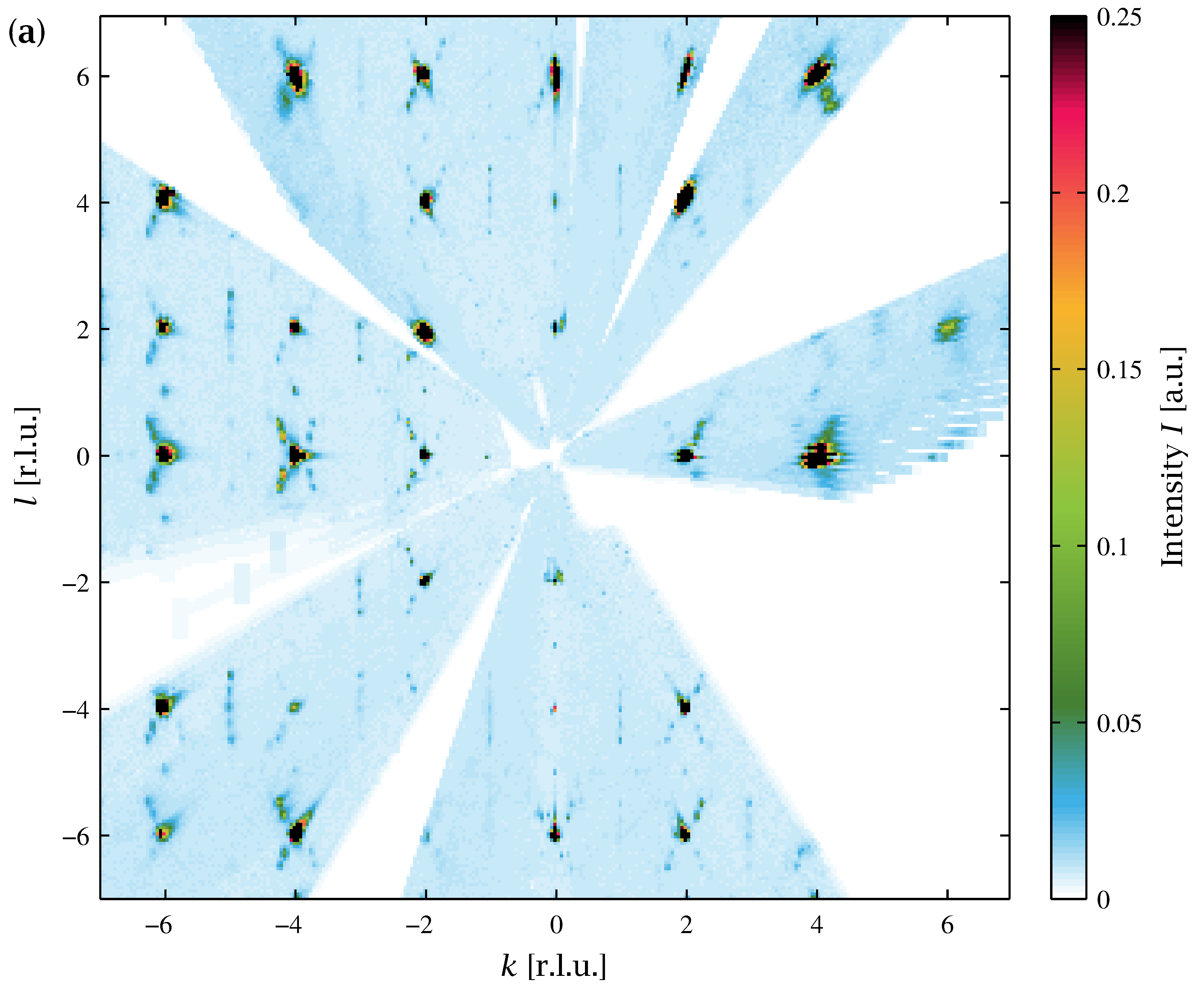
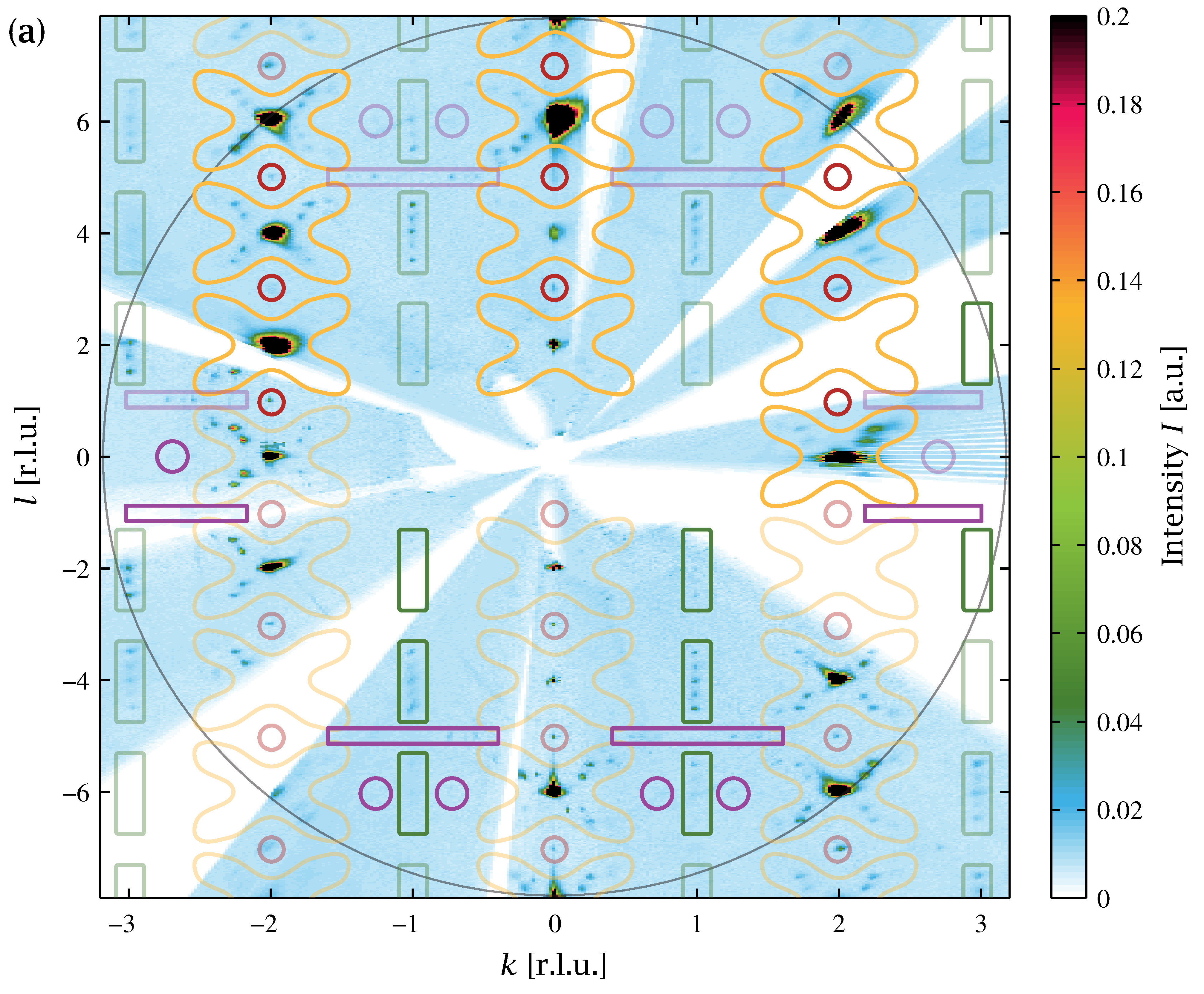
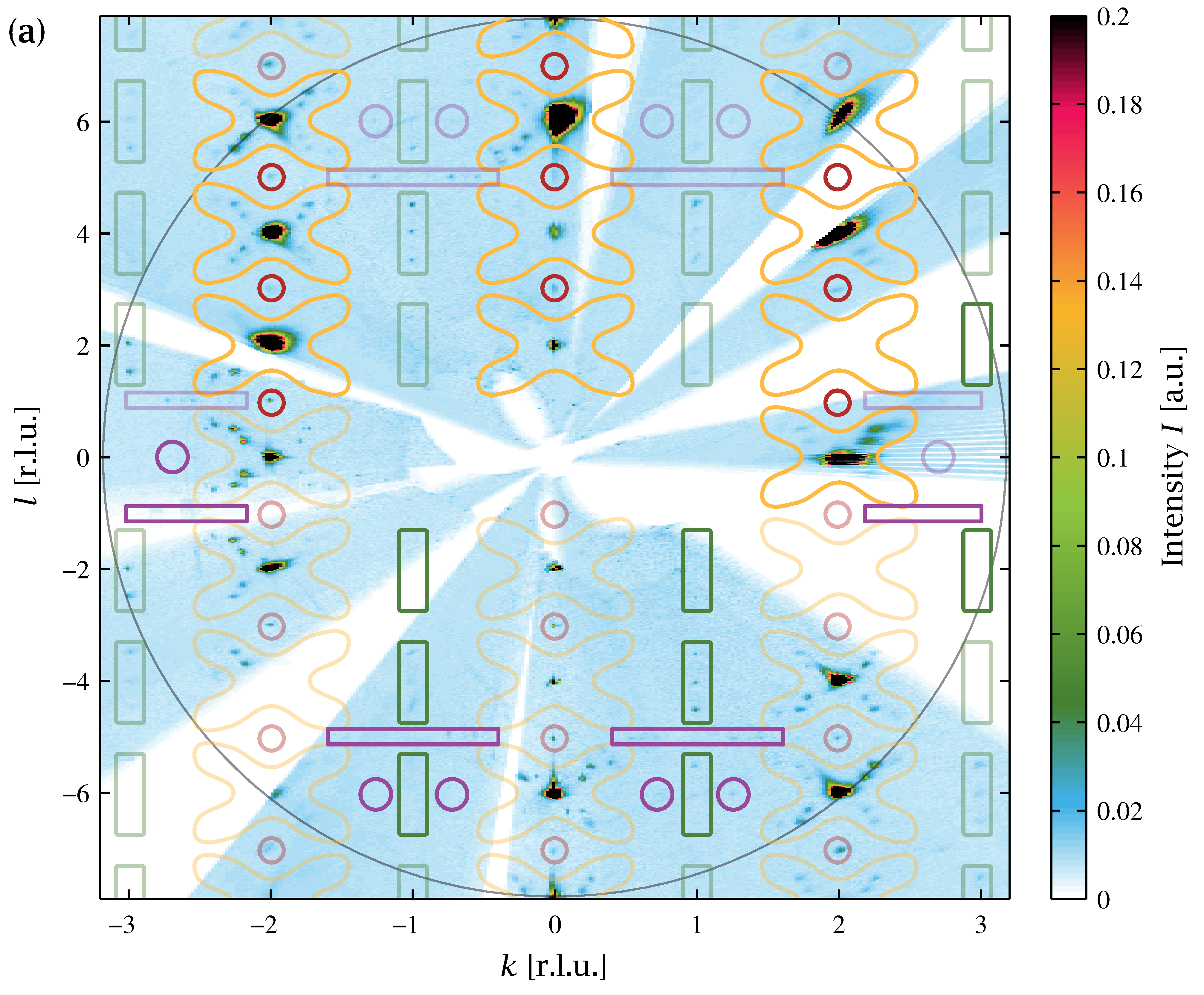
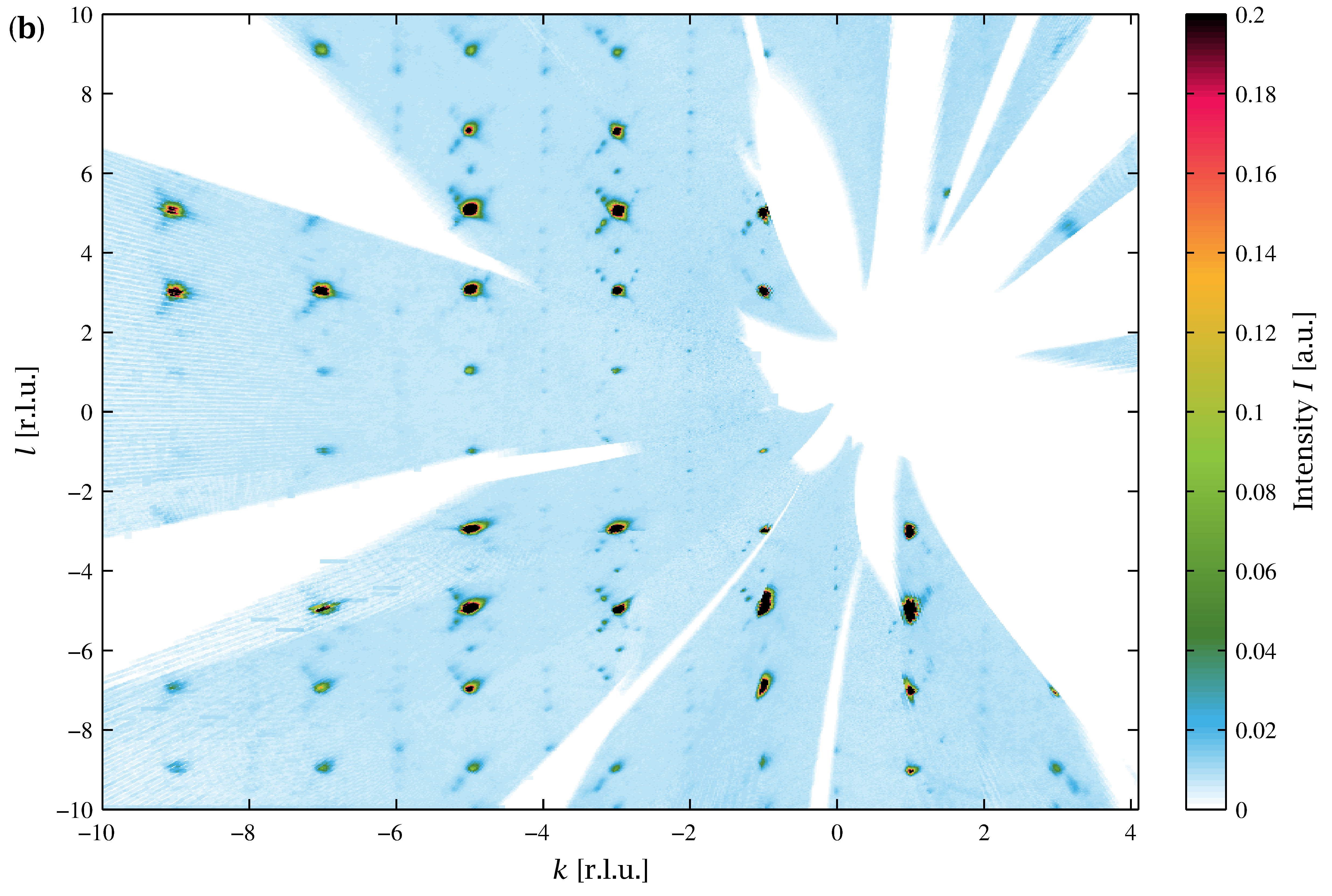
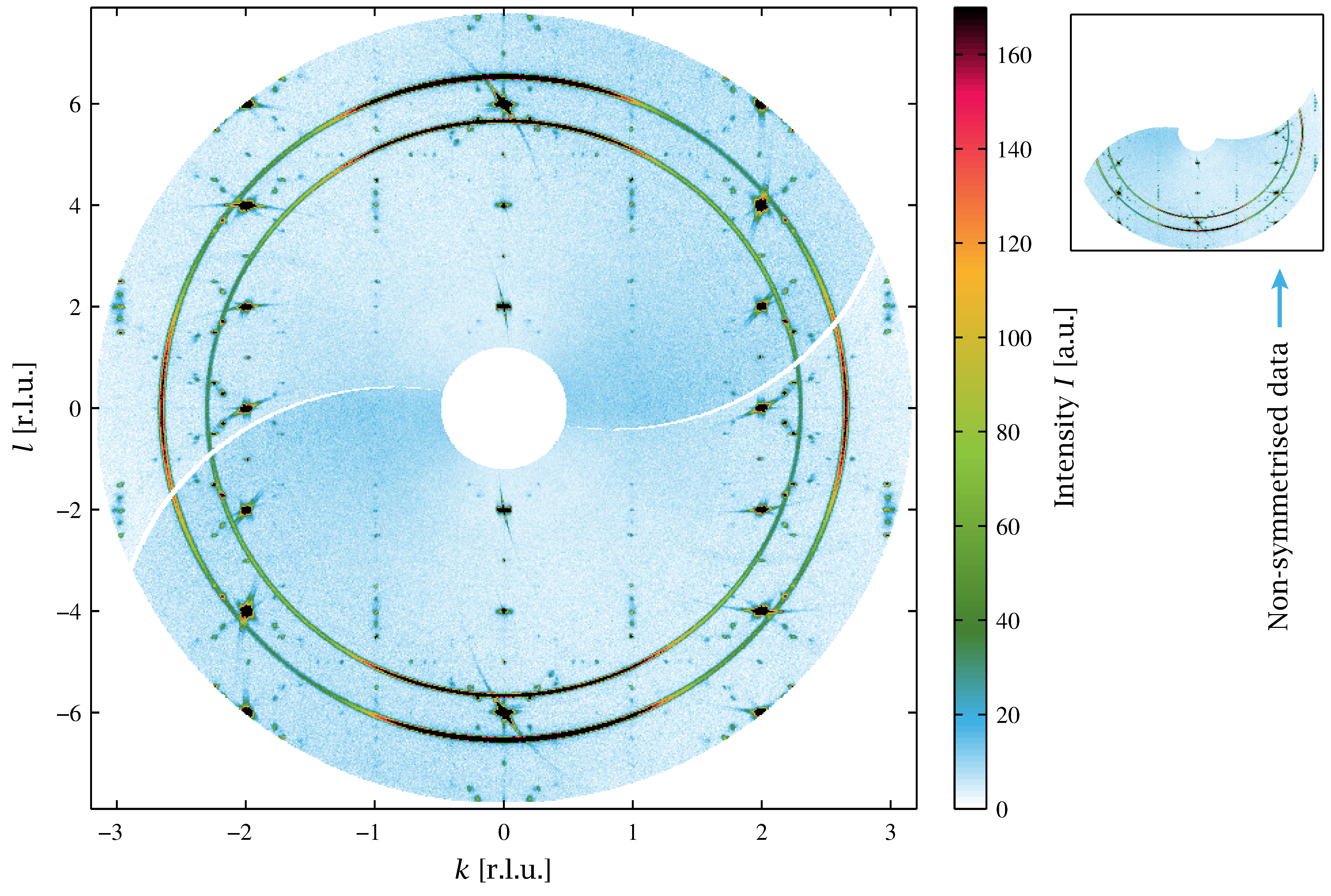
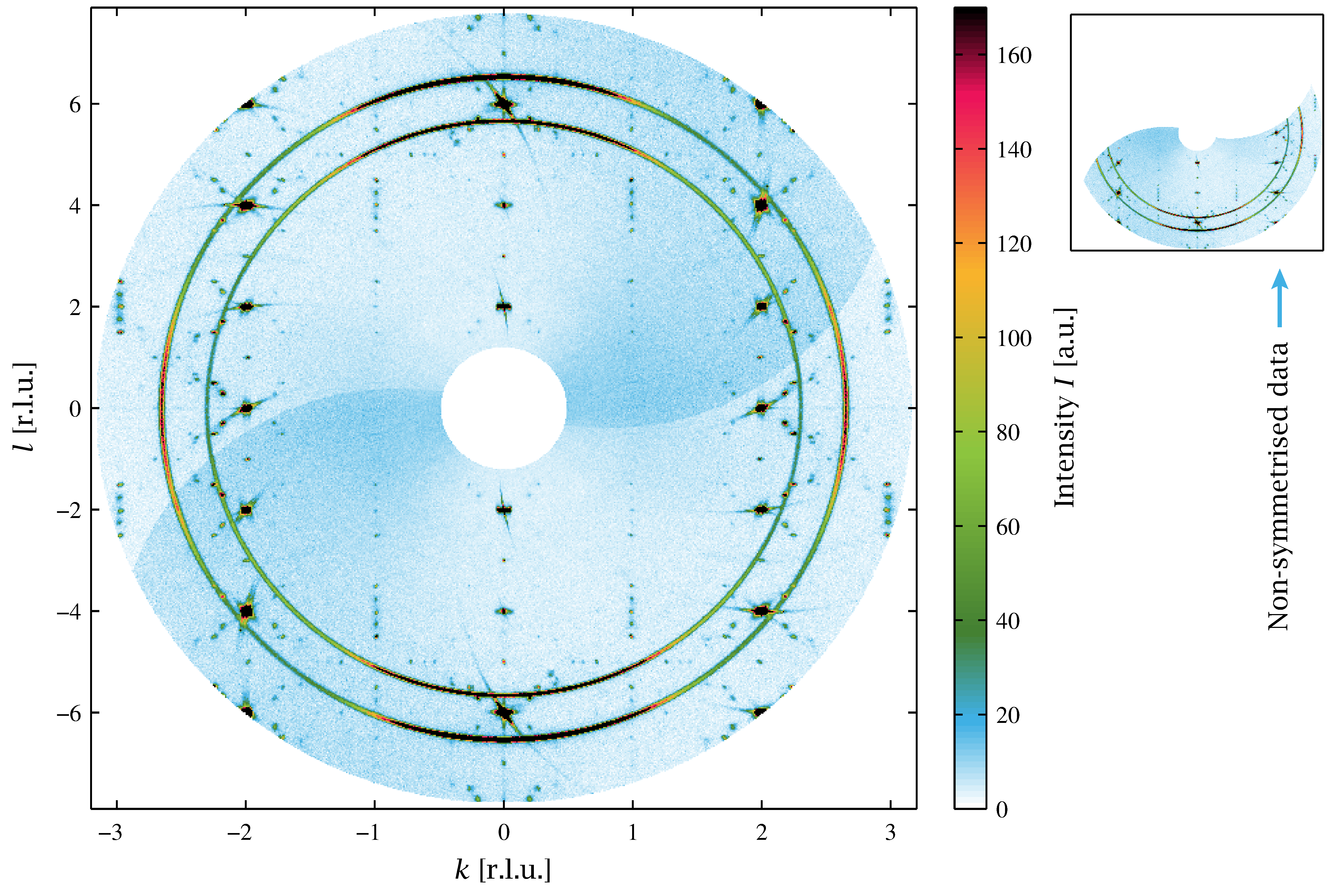
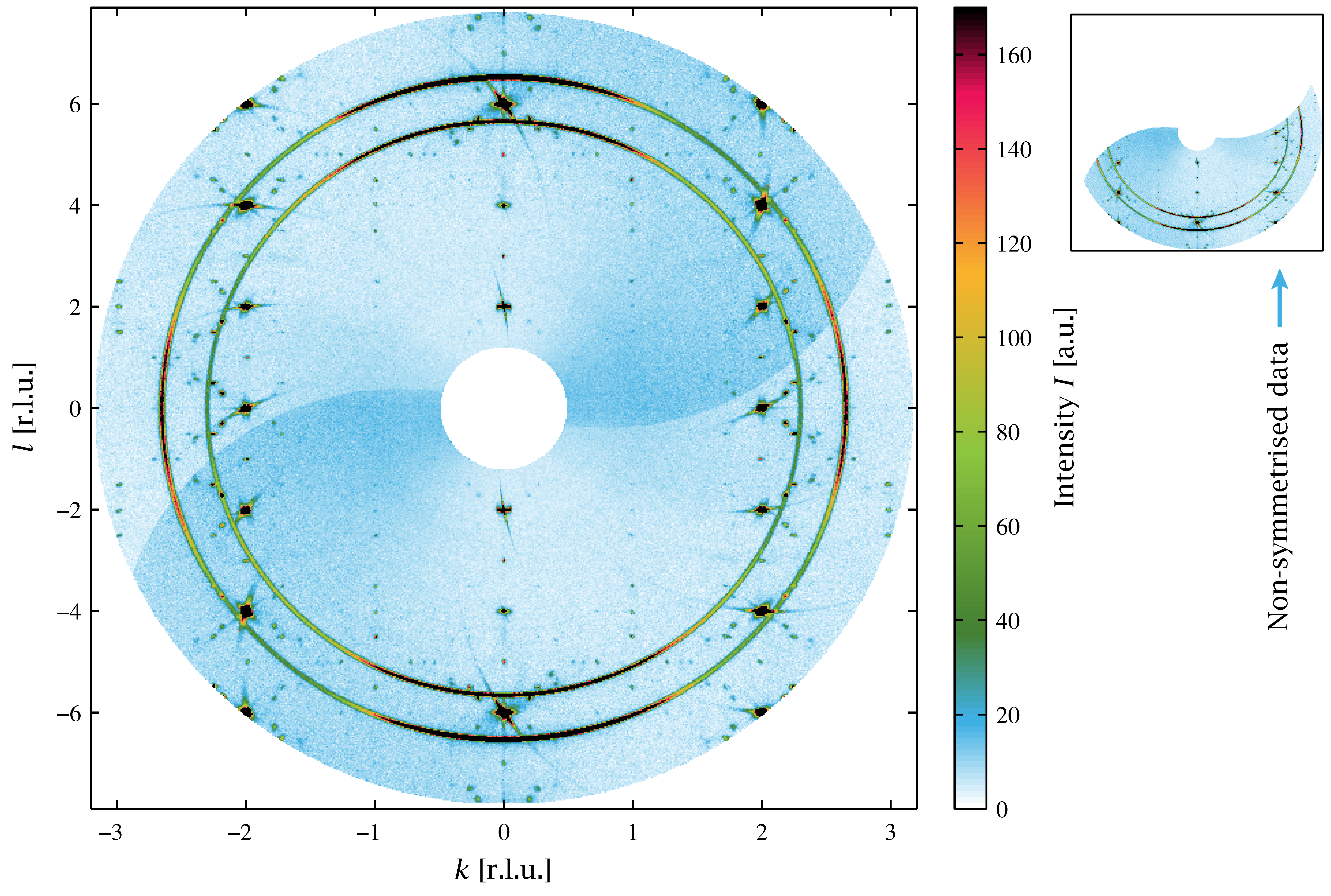
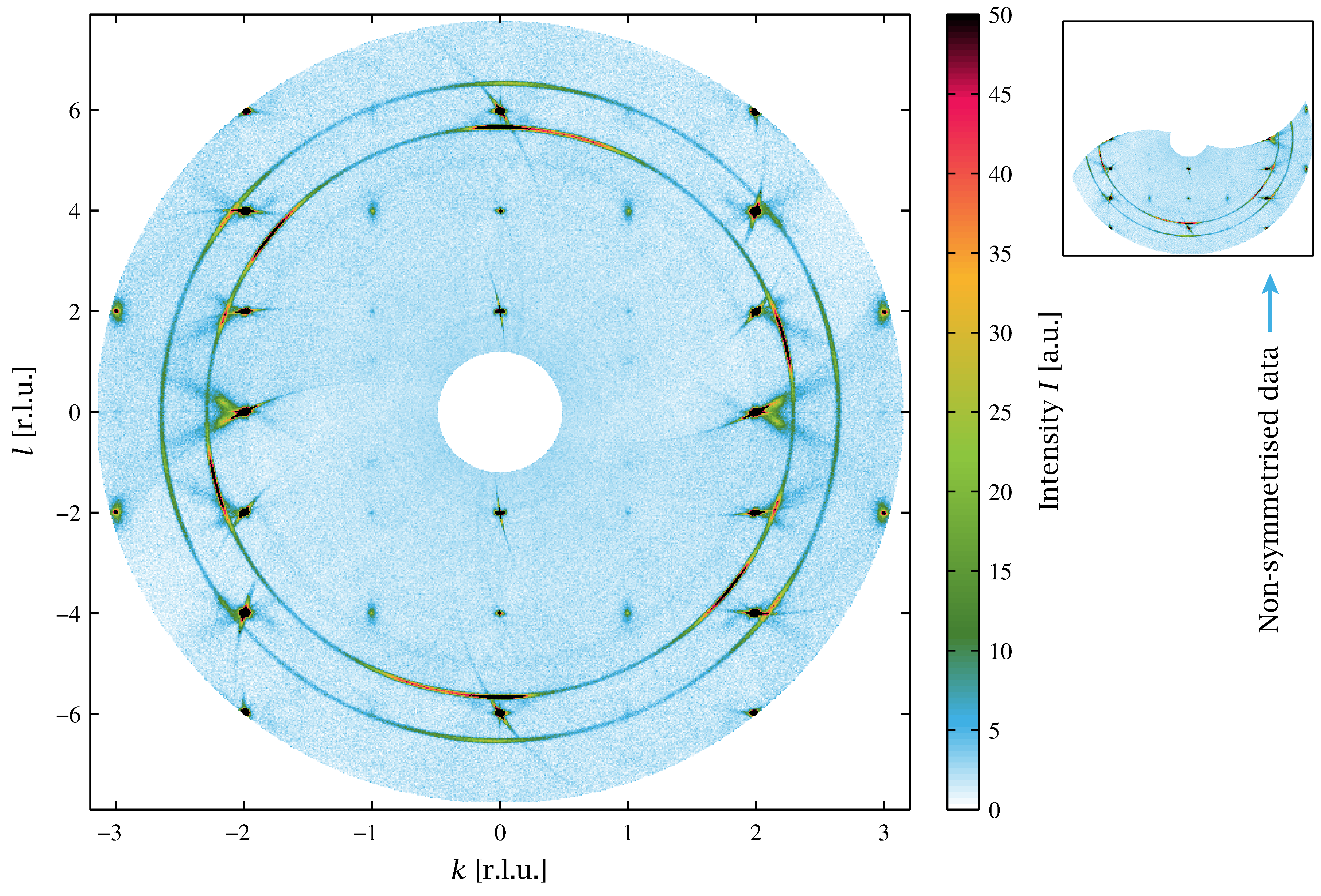
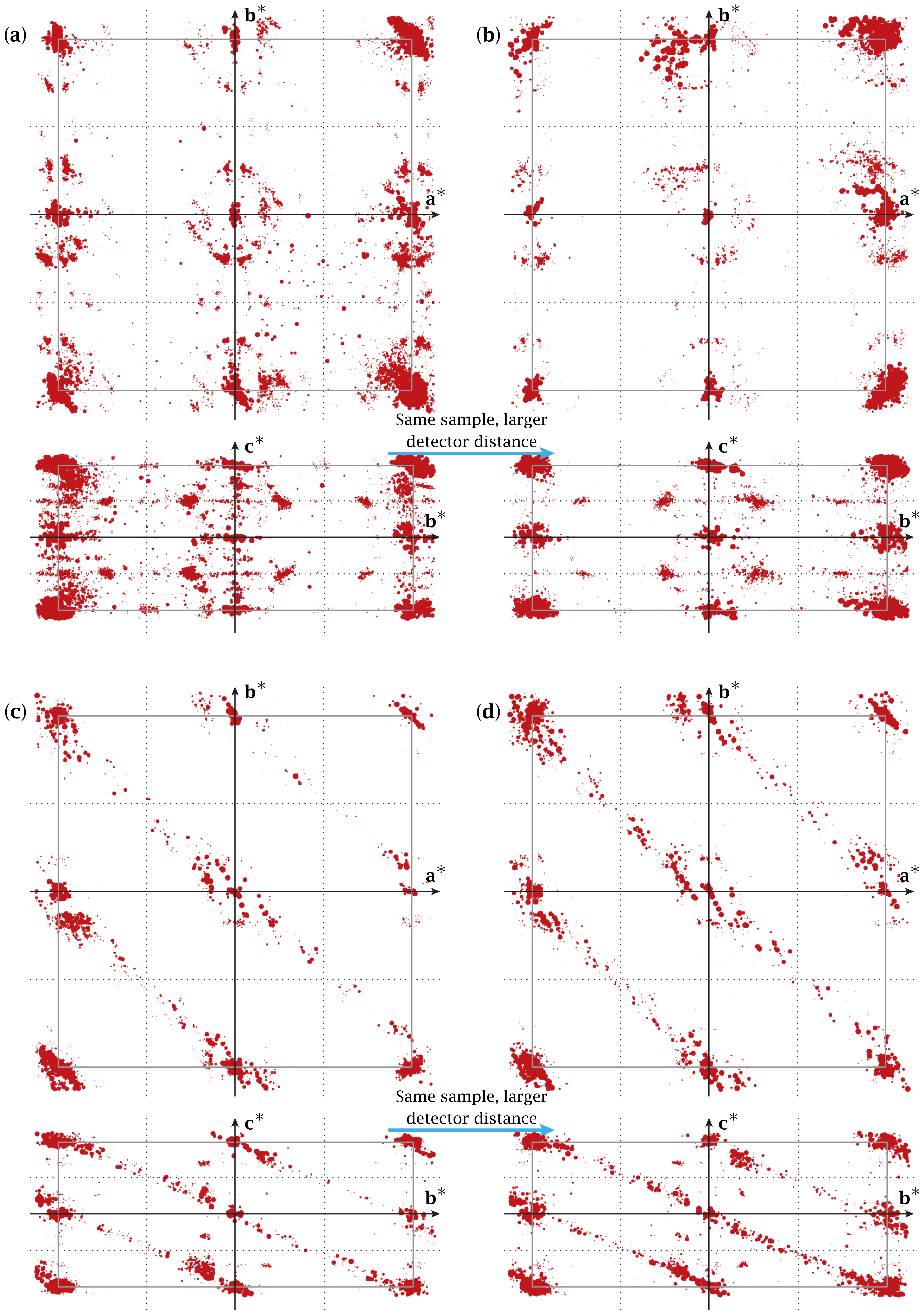
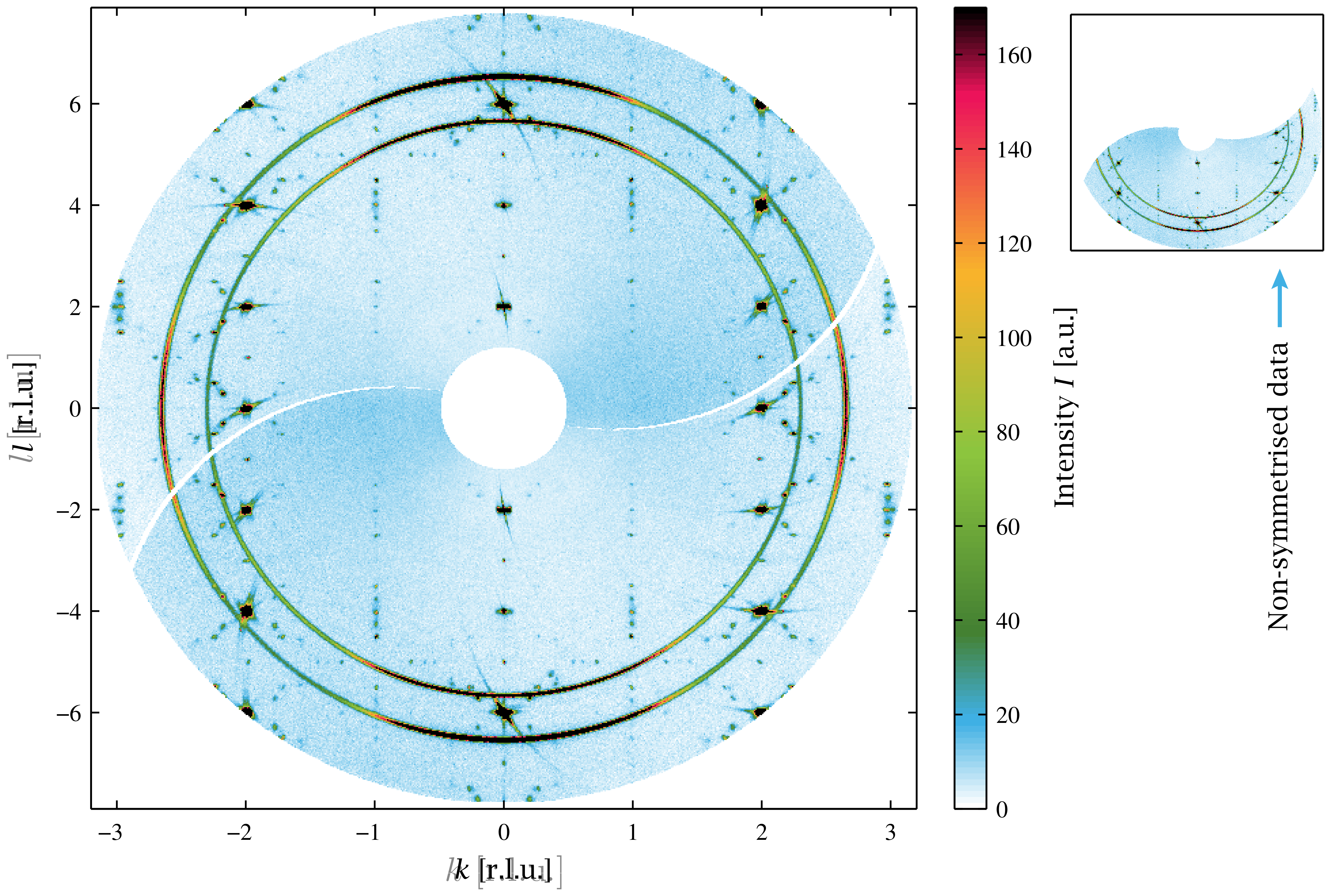
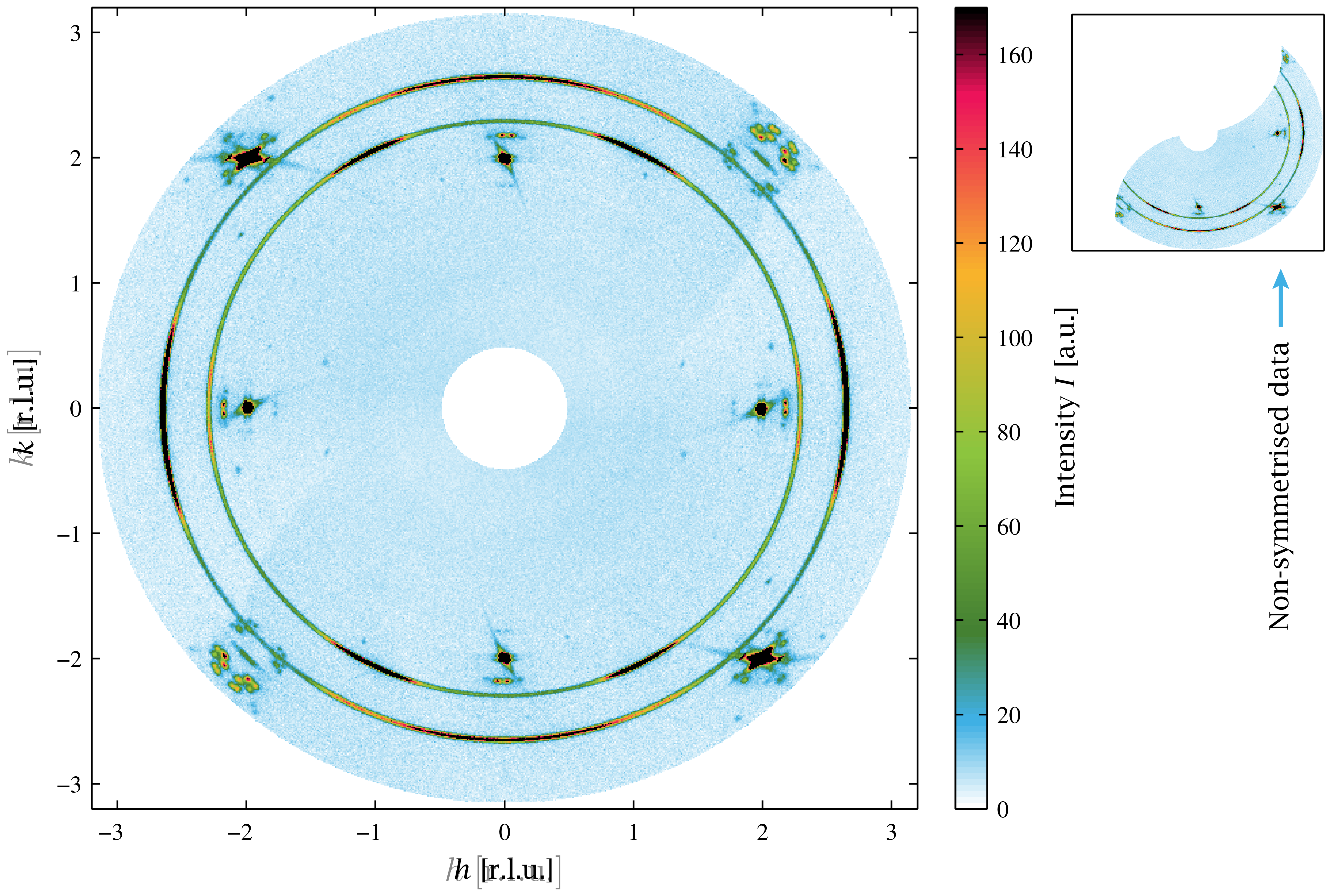
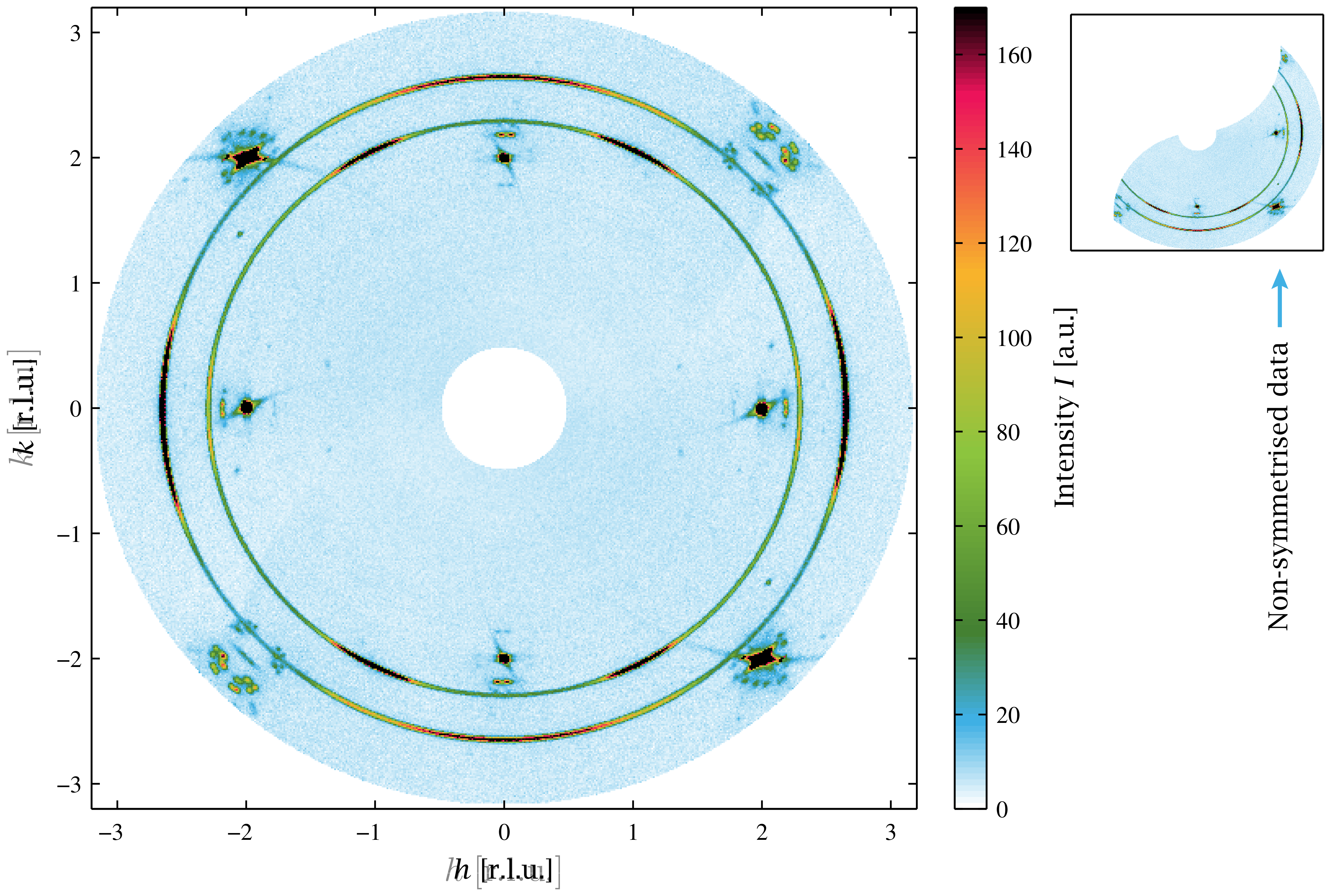
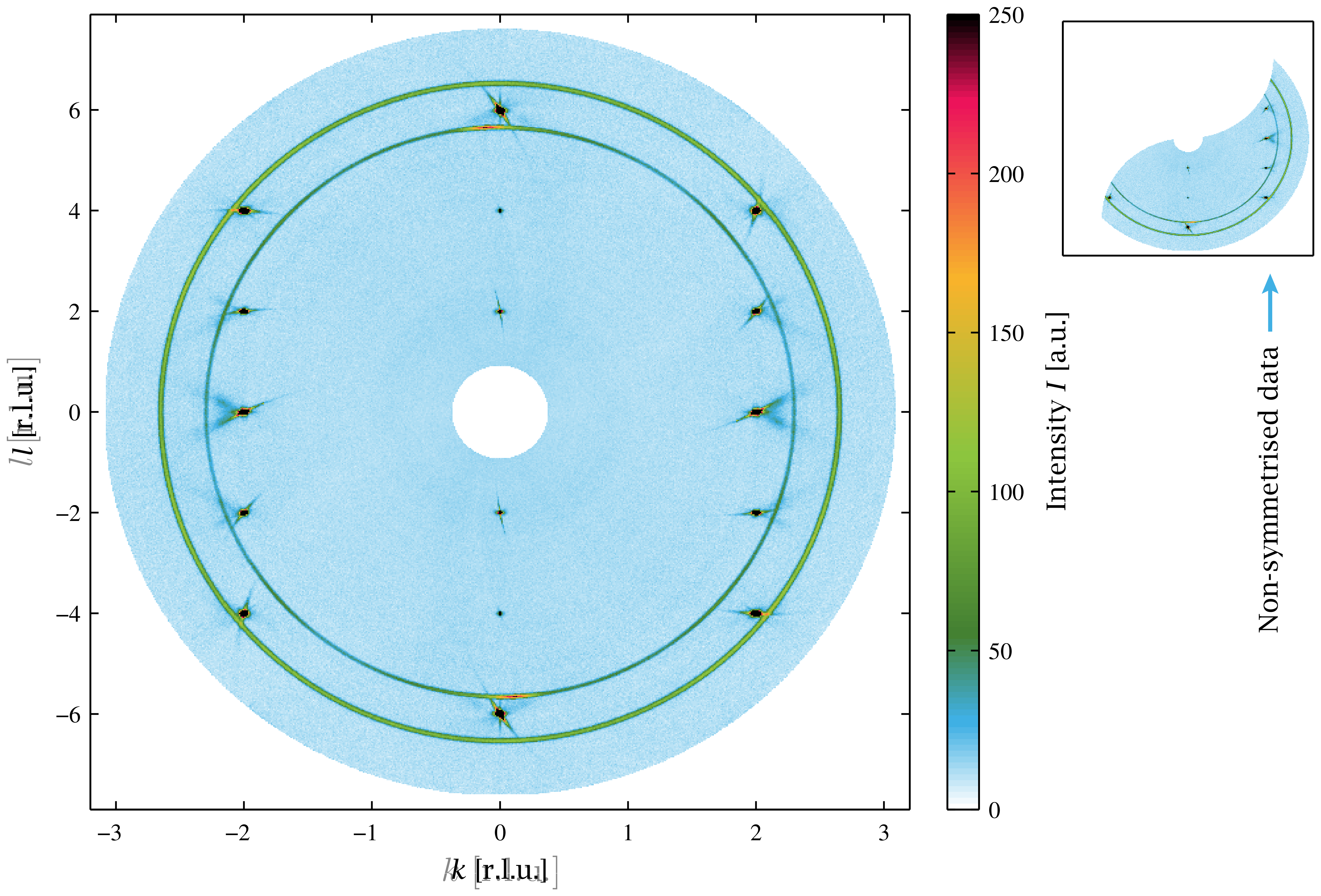
Figur 9.5(a): Example of unwarped (0kl) planes from SXD at 10 K (non-symmetrised). Download links:PNG • SVG (fuld vektor SVG) • PDF (fuld vektor PDF). .
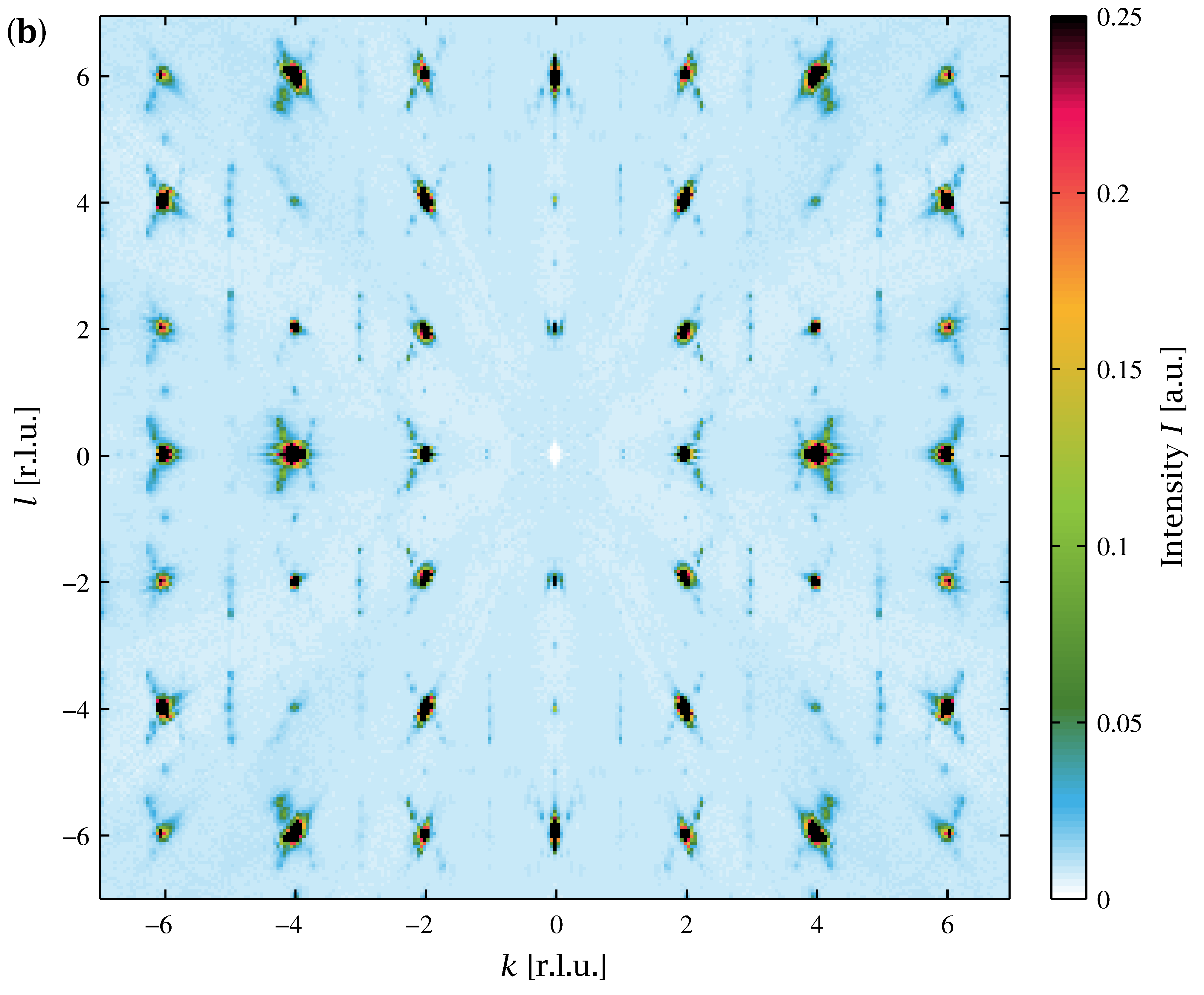
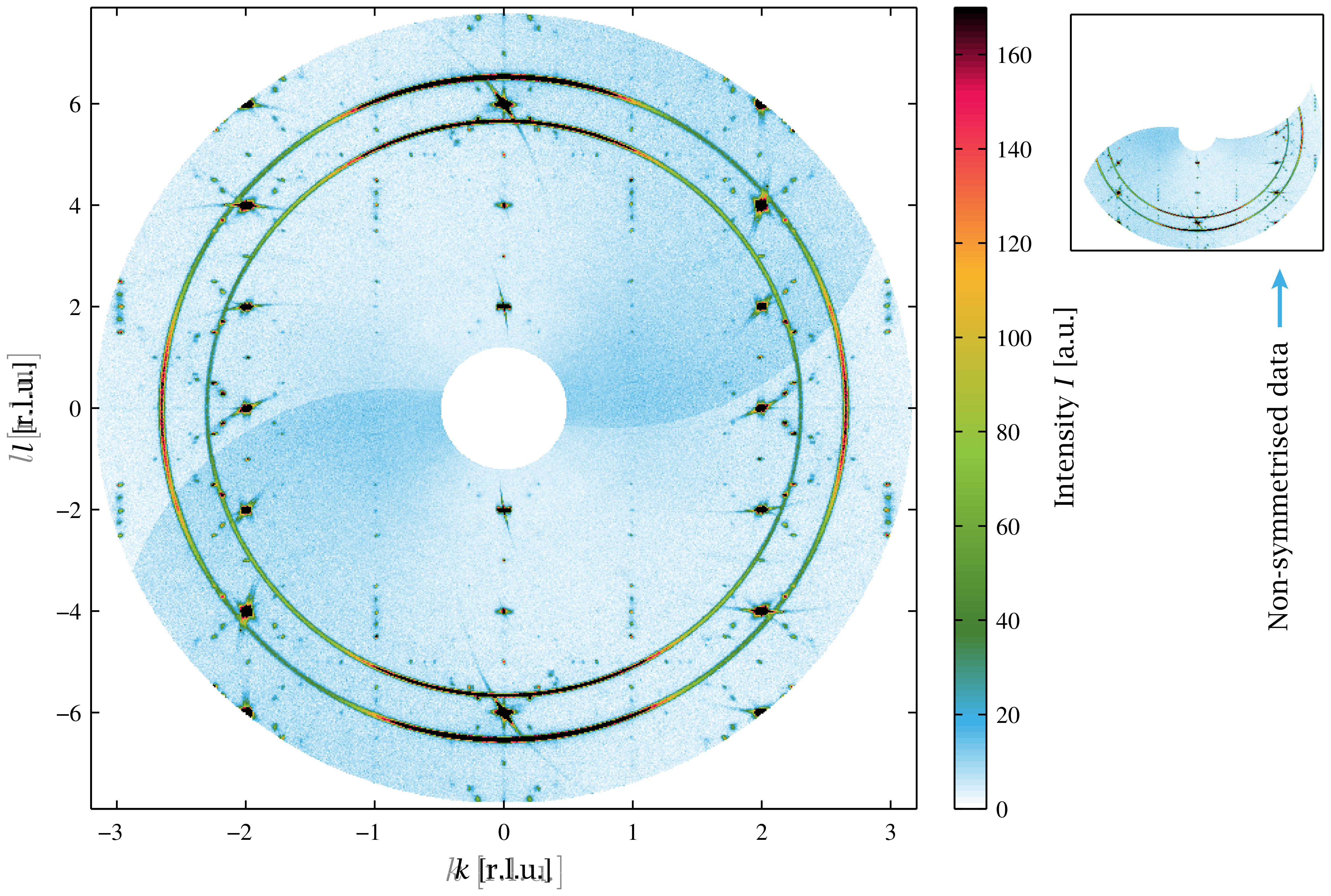
Figur 9.5(b): Example of unwarped (0kl) planes from SXD at 10 K (symmetrised). Download links:PNG • SVG (fuld vektor SVG) • PDF (fuld vektor PDF). .
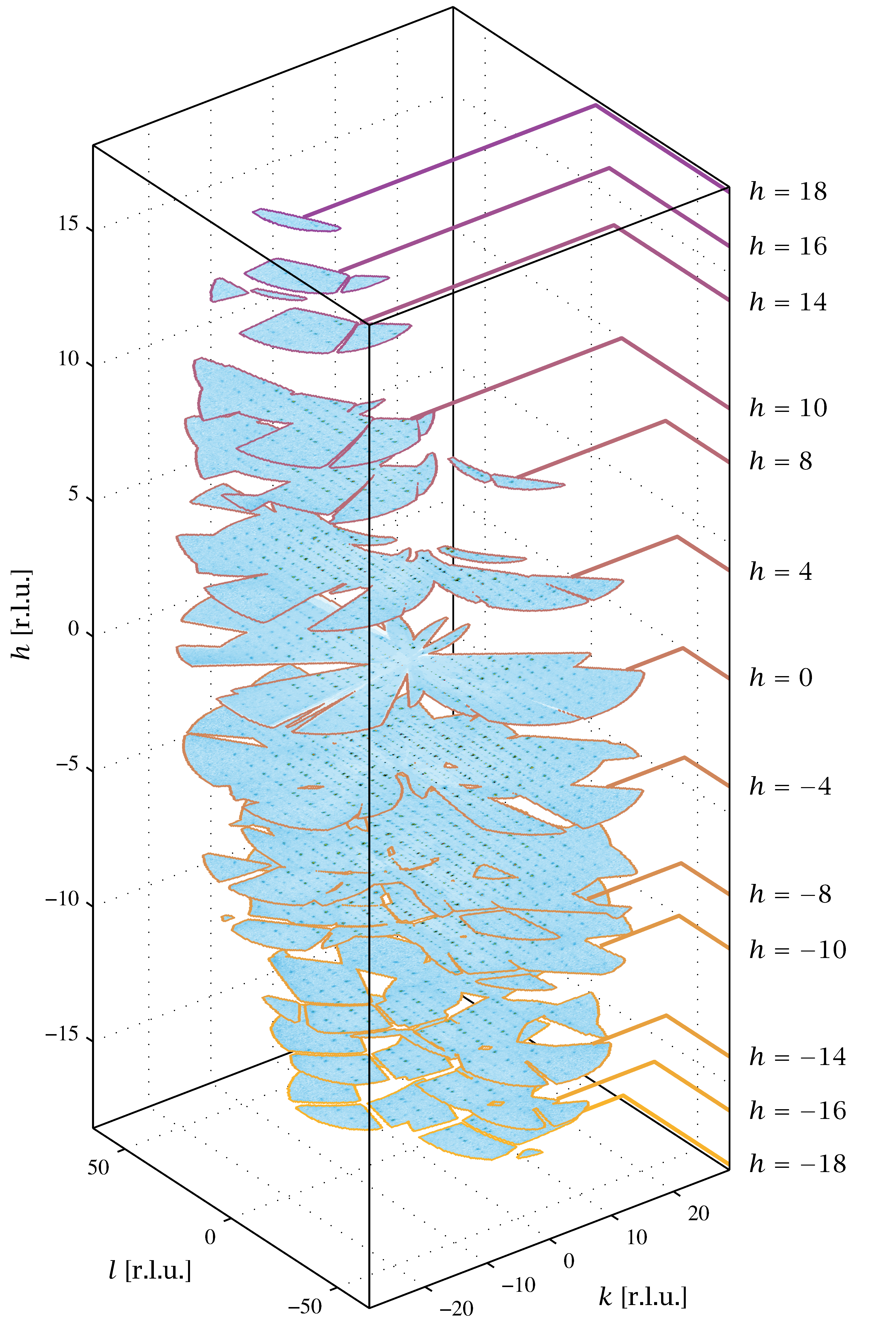
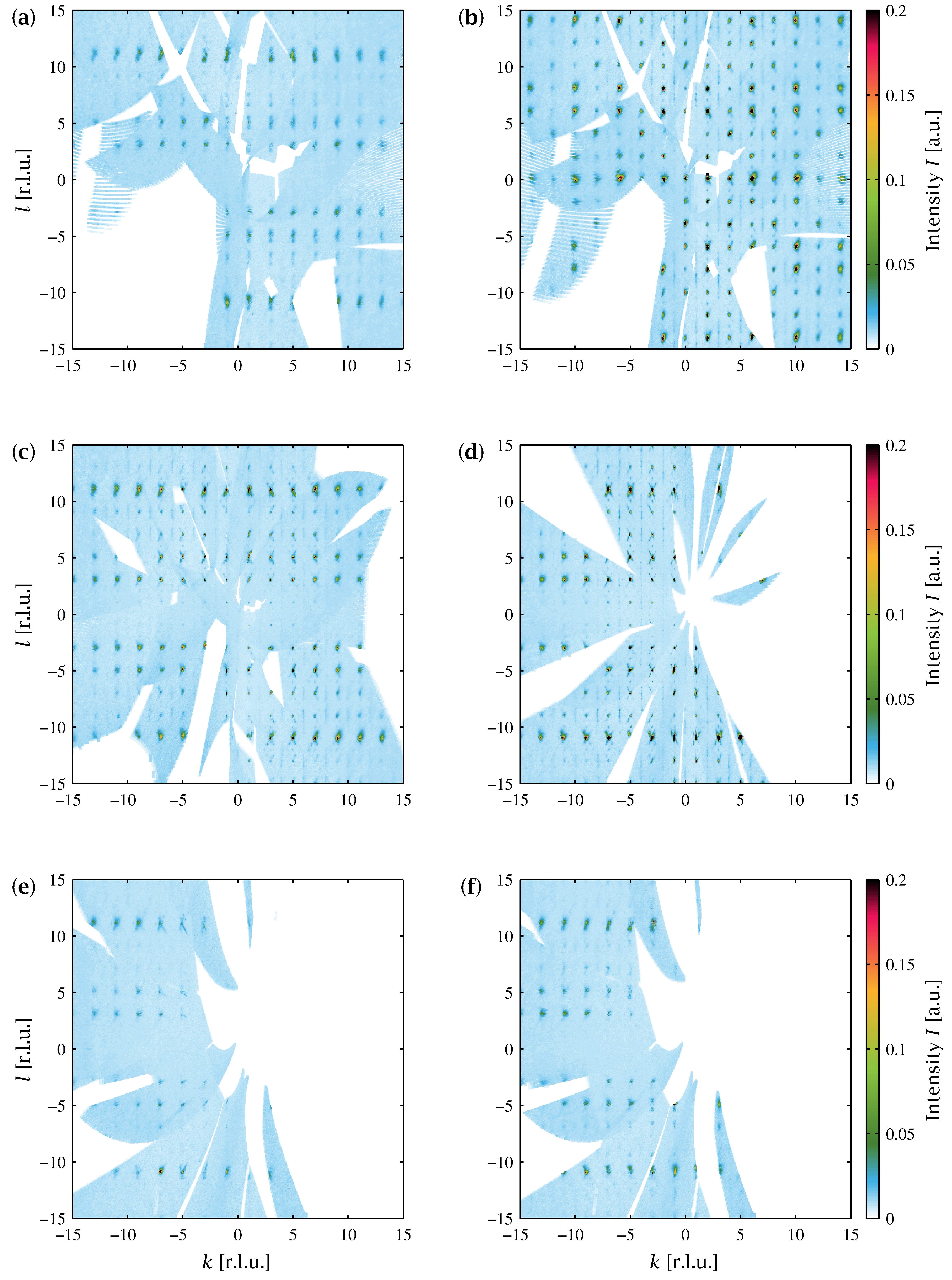
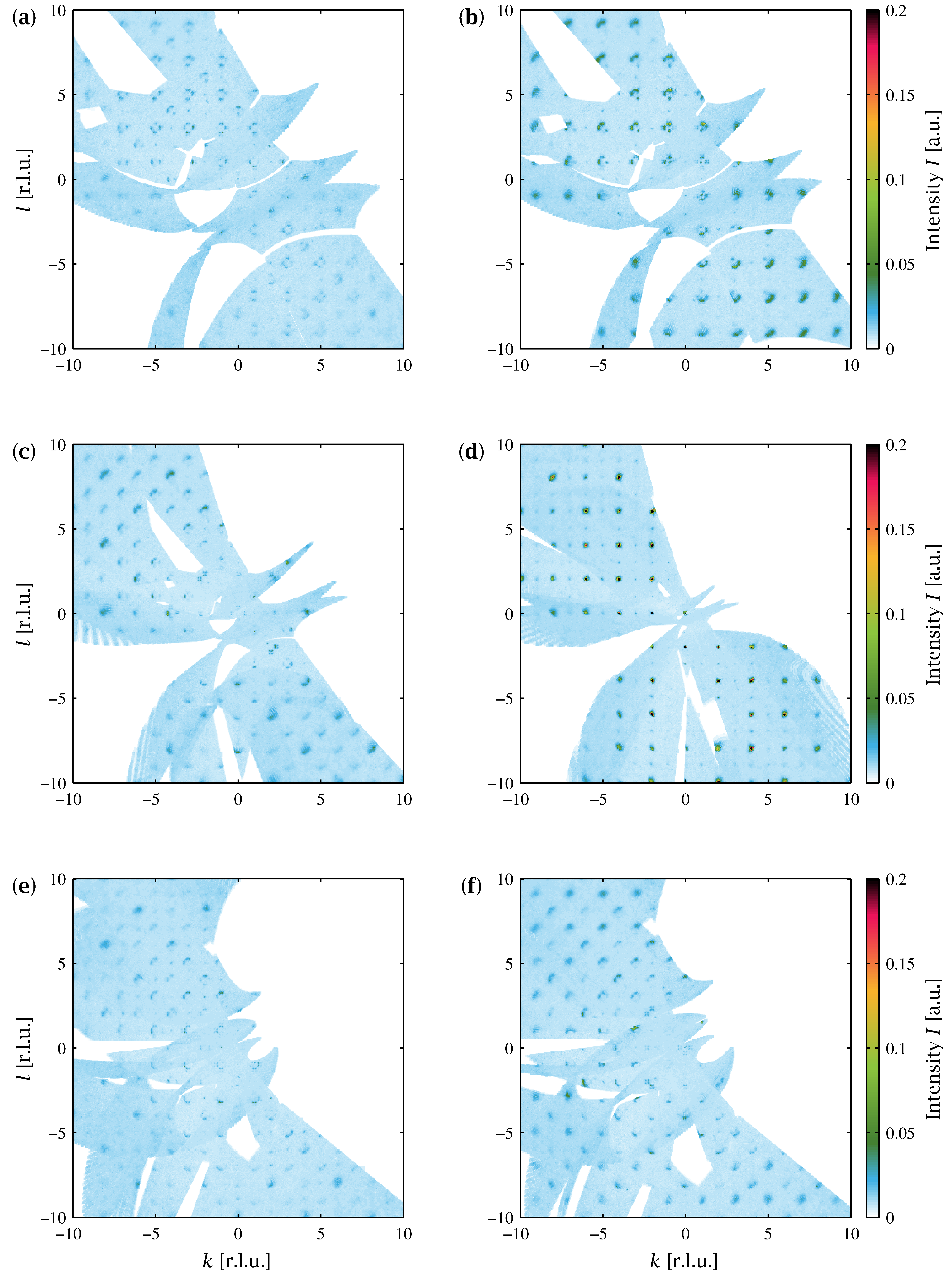
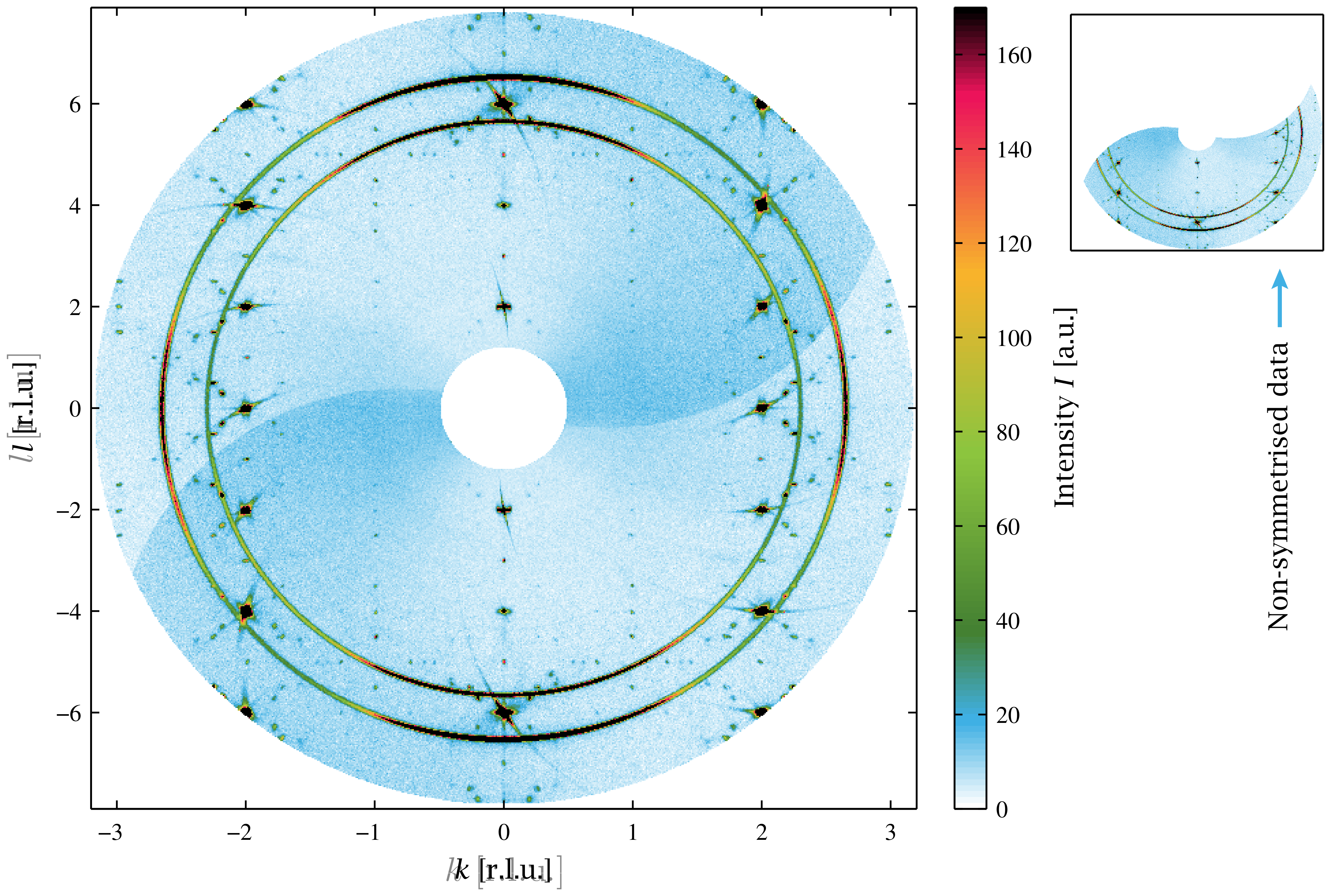
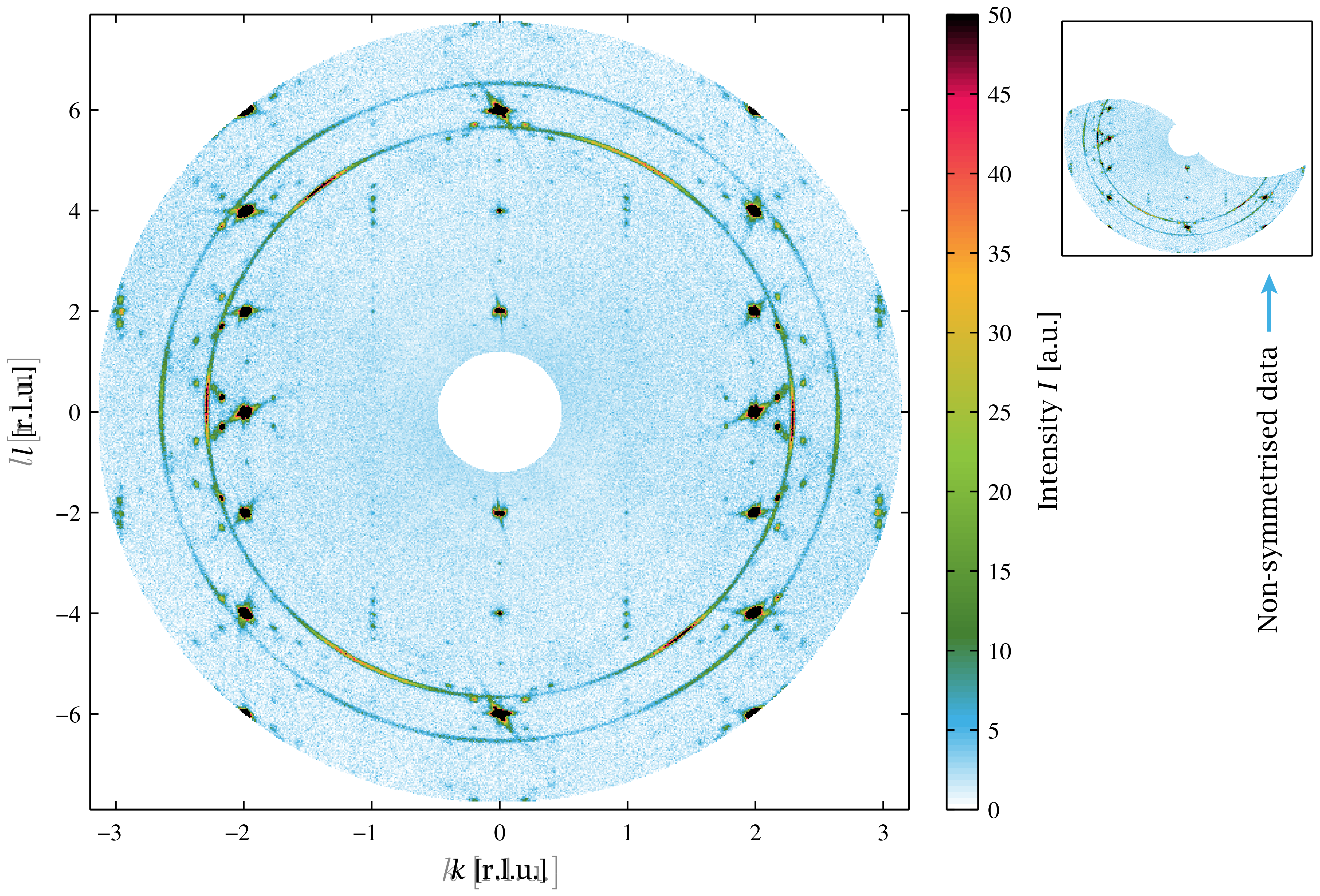
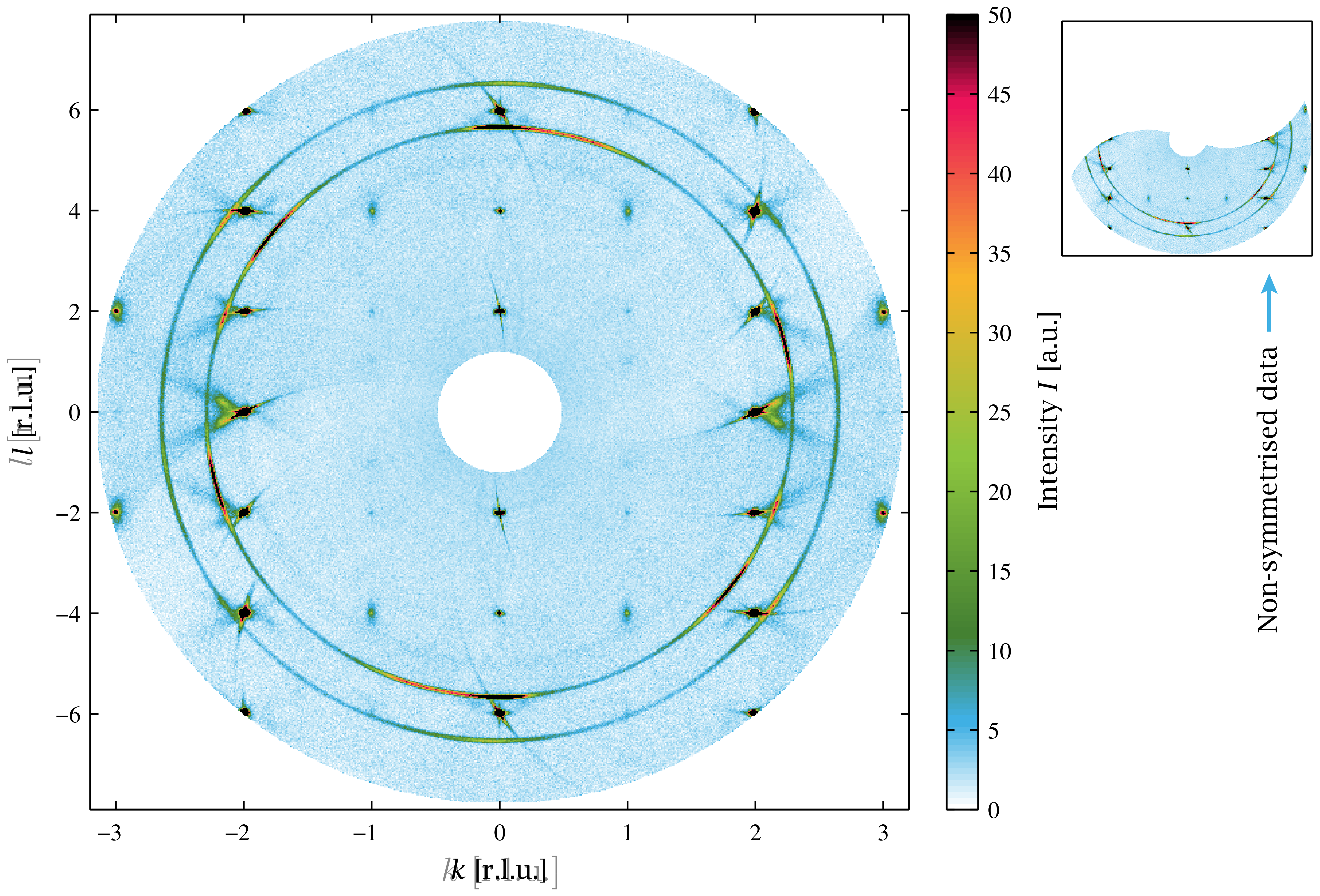
Figur 9.6: Unwarped kl planes at varied h - showing volume on SXD. Download links:PNG • SVG (fuld vektor SVG) • PDF (fuld vektor PDF). .
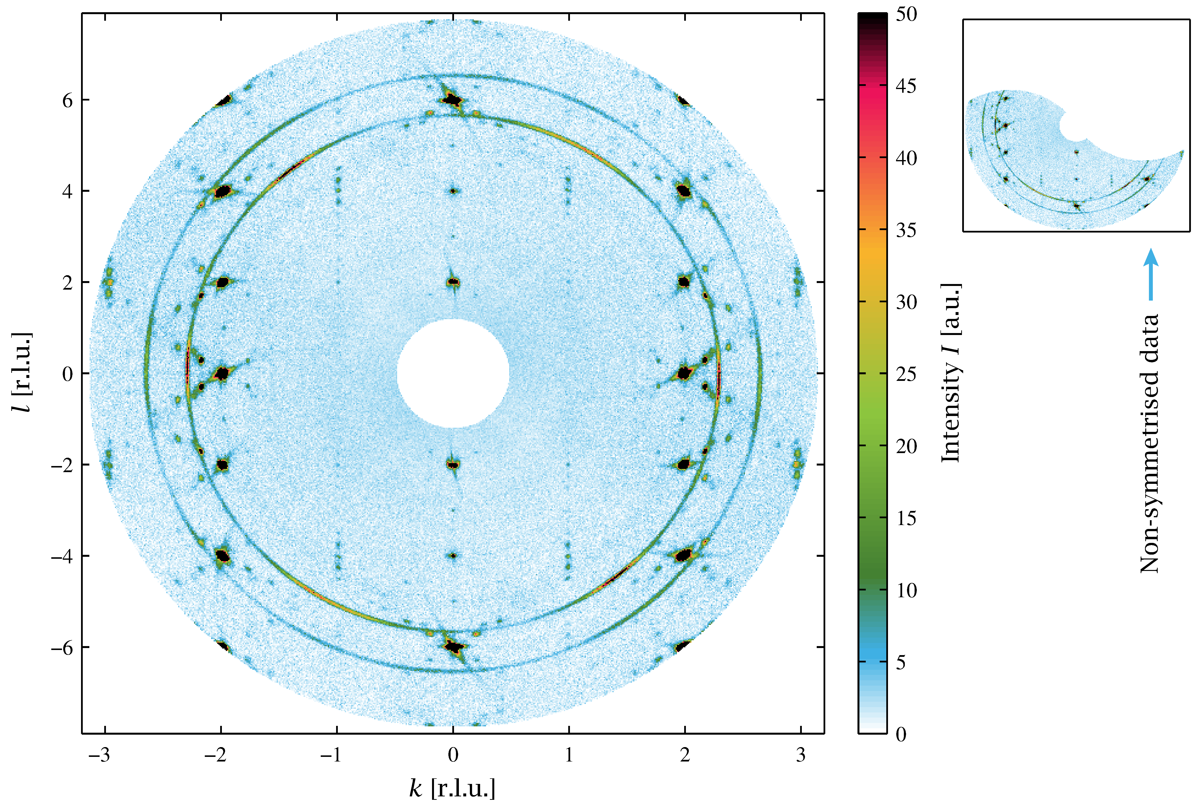
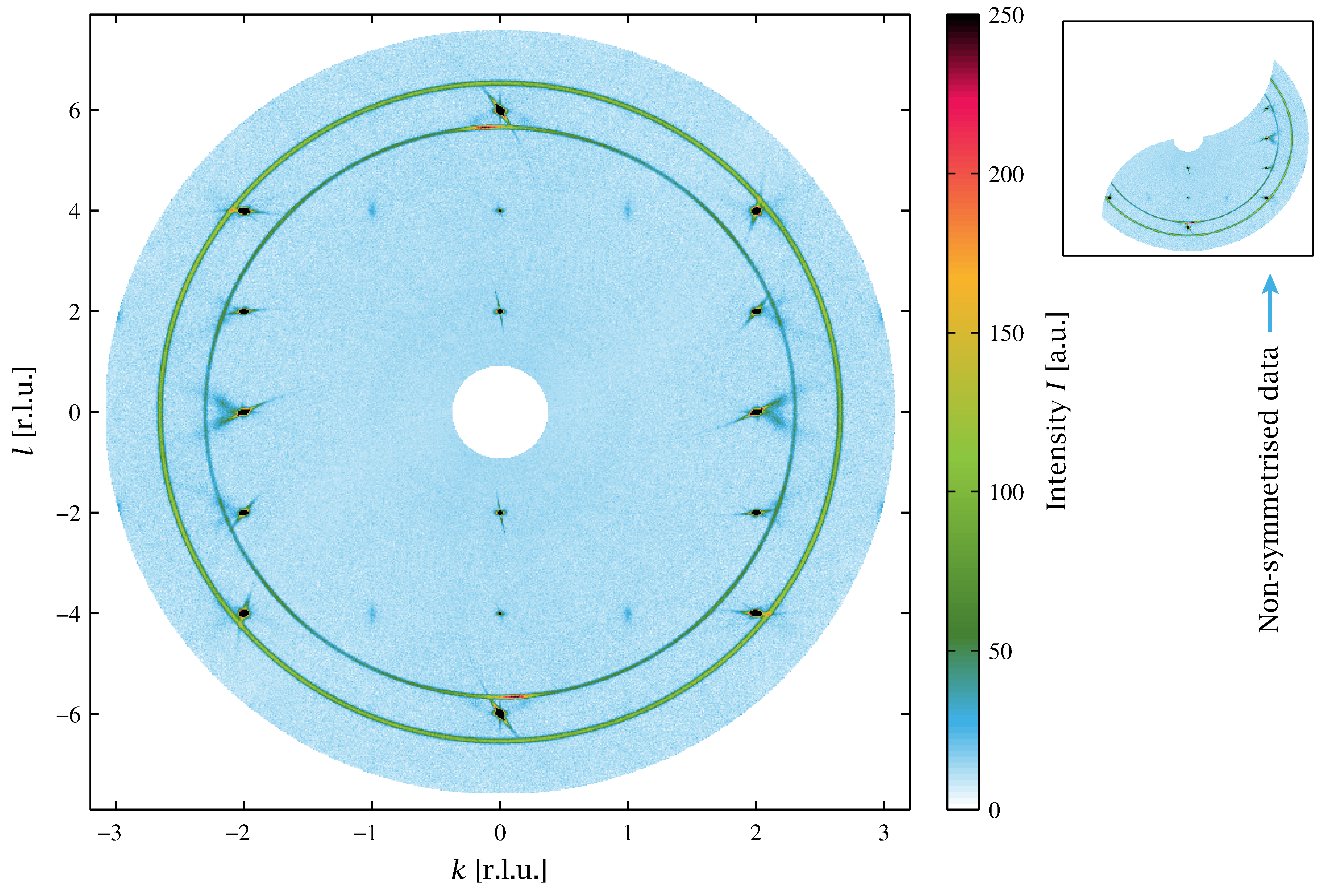
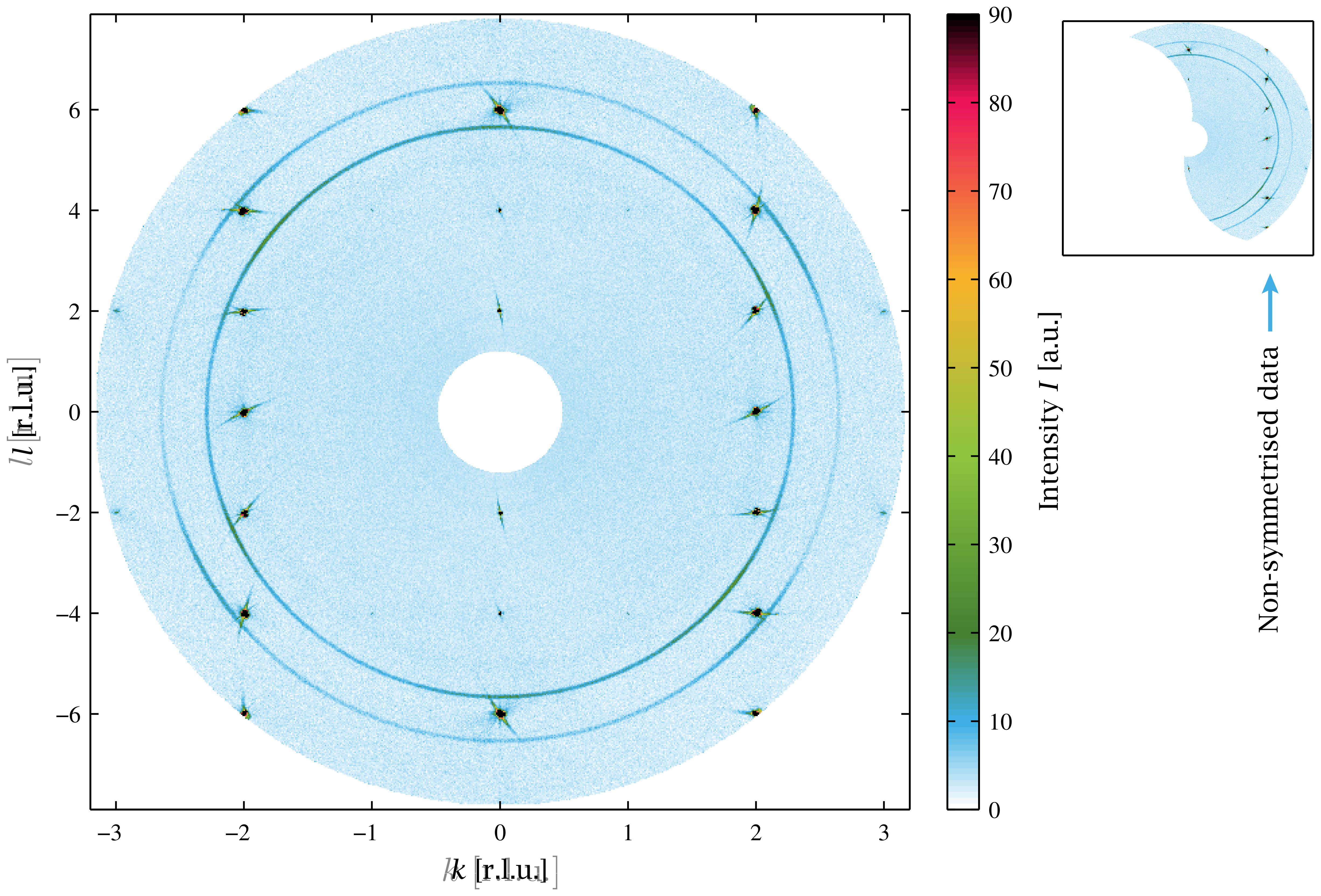
Figur 9.7(a): DMC comparison plots - unwarped (0kl) SXD plane at 10 K. Download links:PNG • SVG (fuld vektor SVG) • PDF (fuld vektor PDF). .
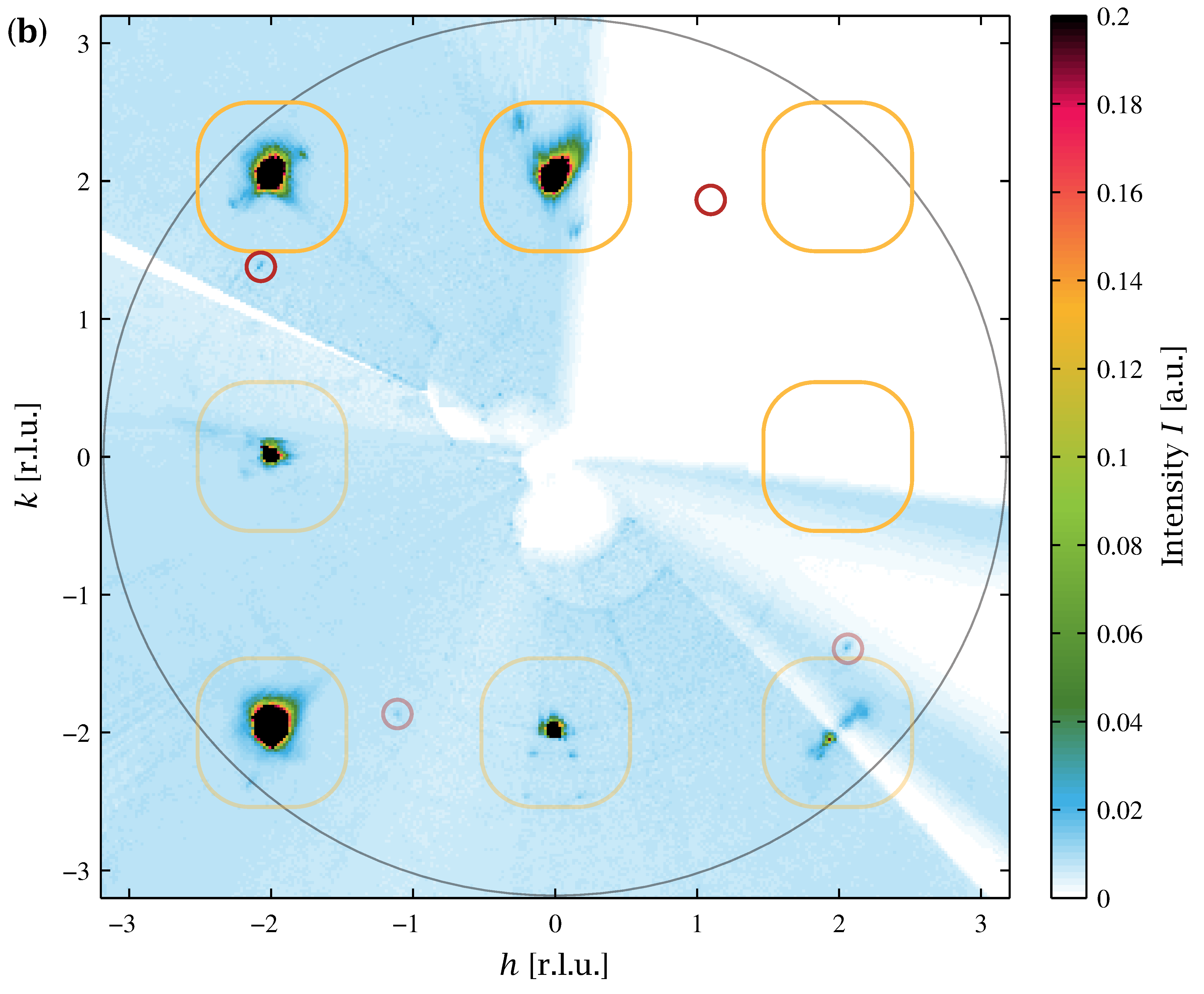
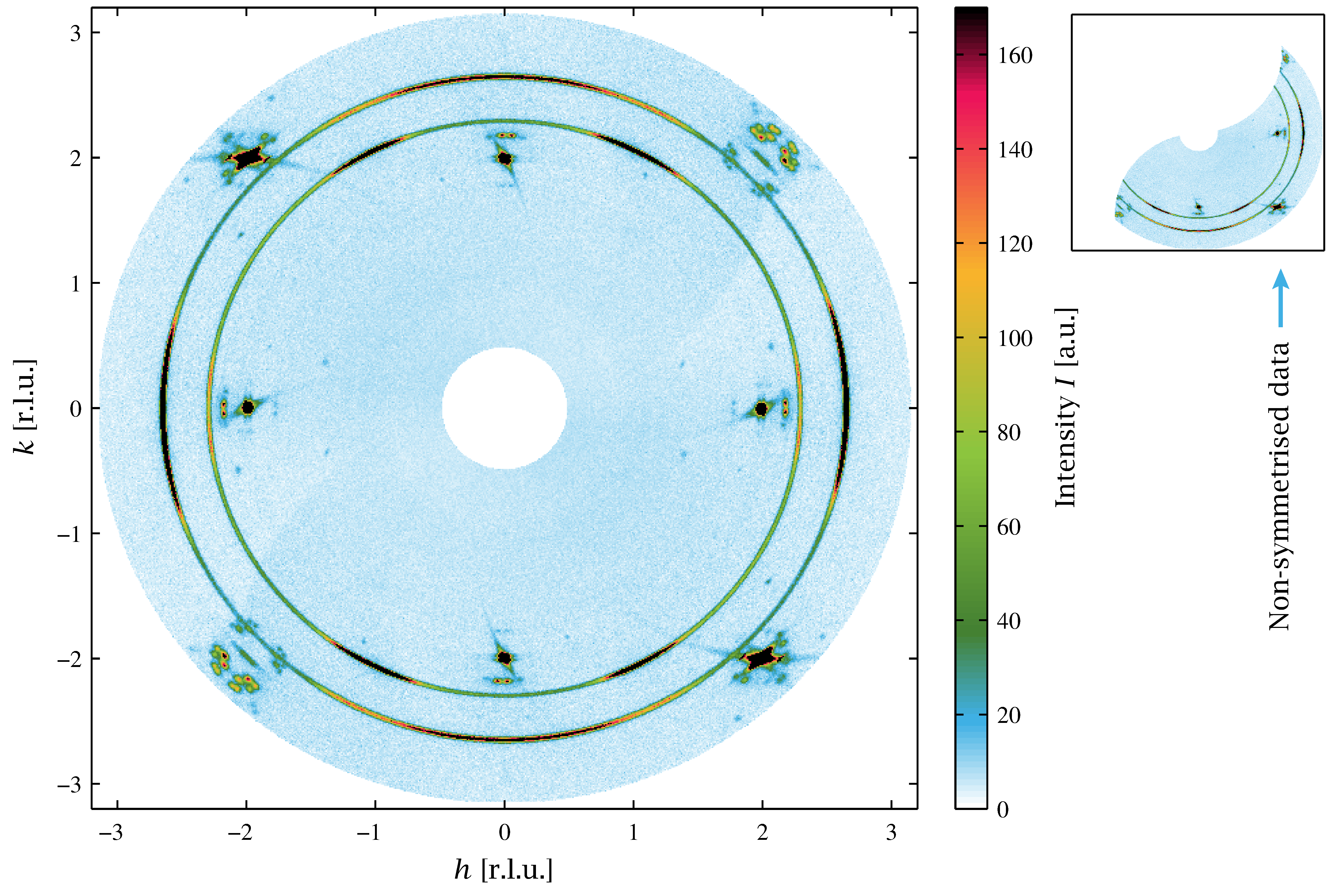
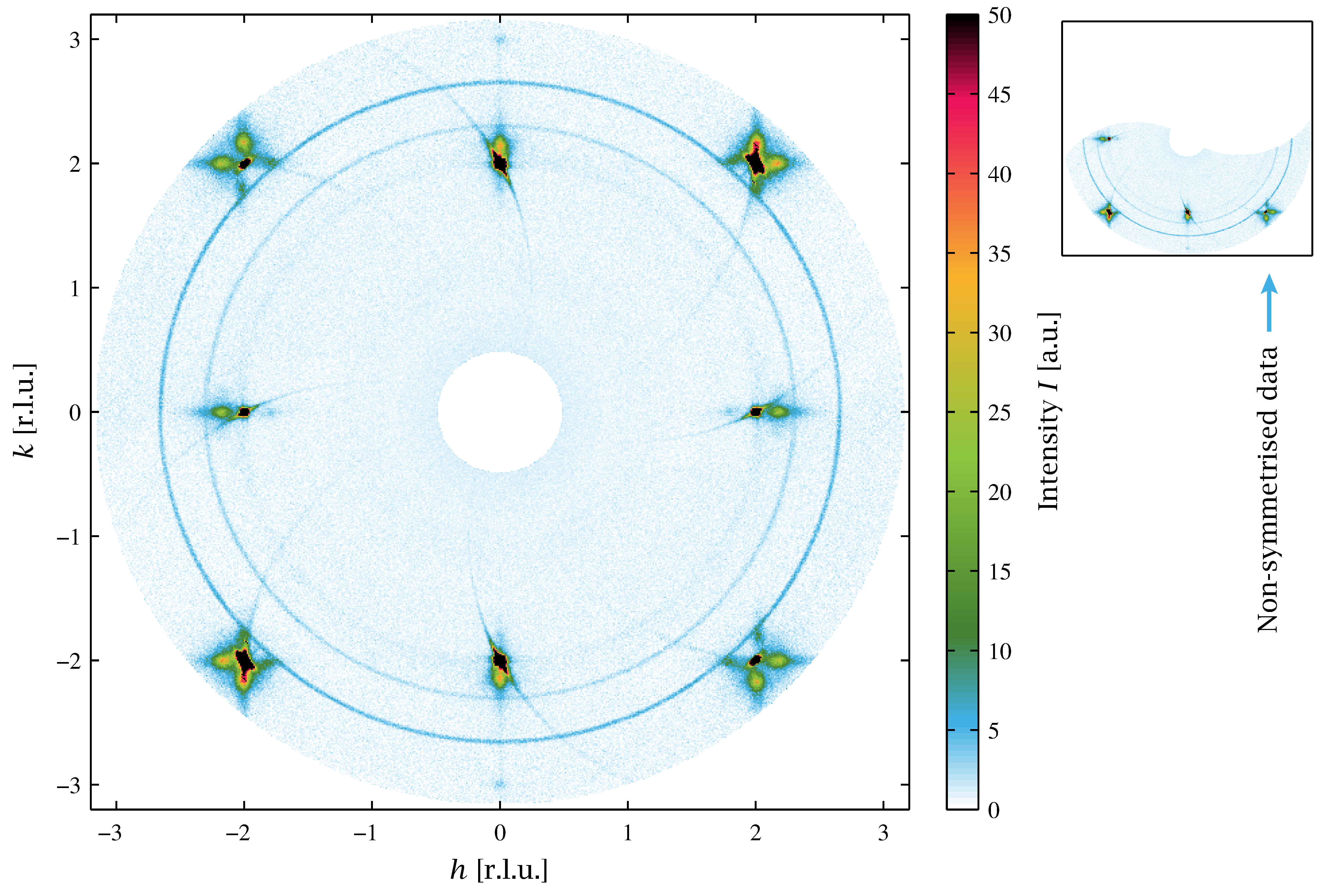
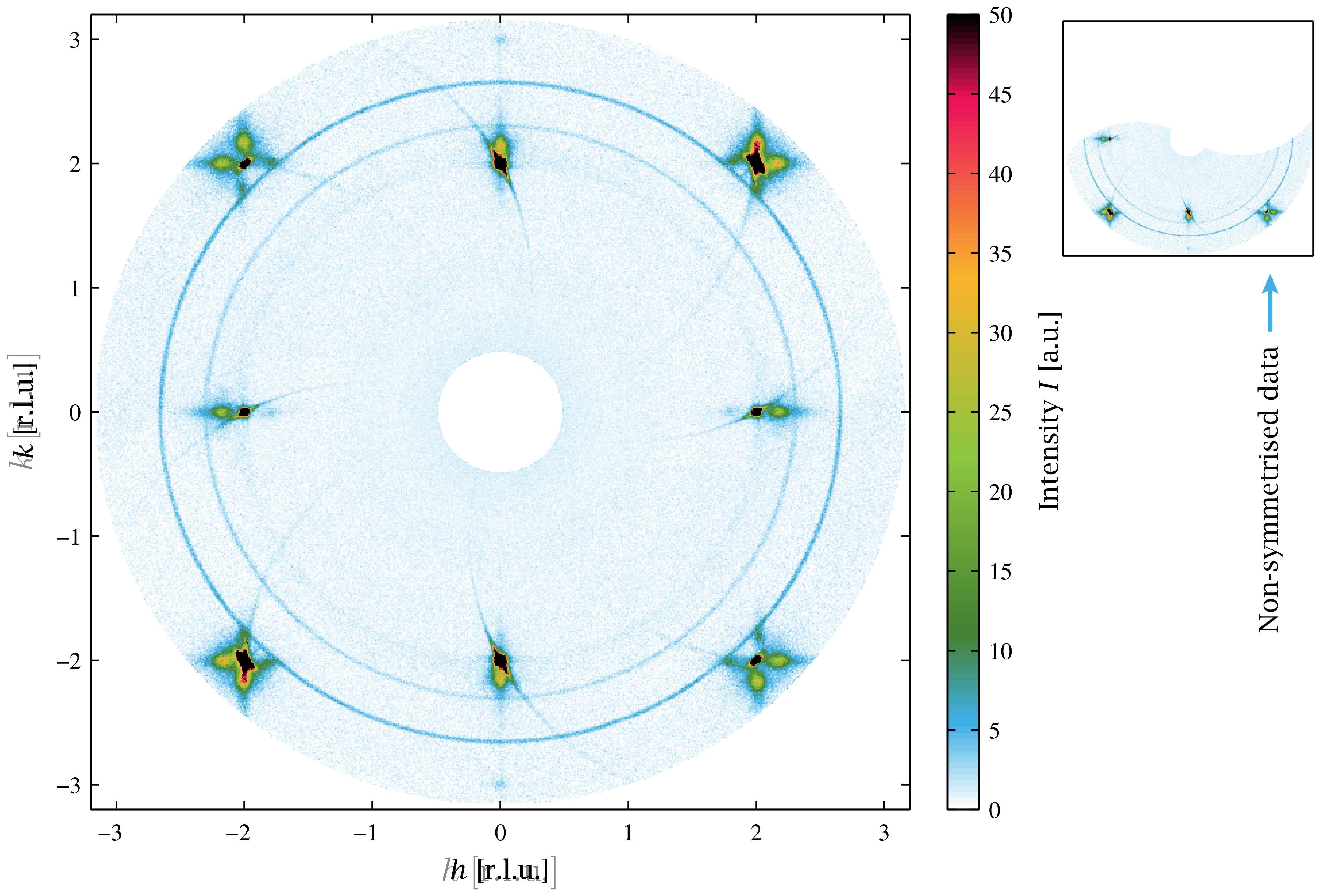
Figur 9.7(b): DMC comparison plots - unwarped (hk0) SXD plane at 10 K. Download links:PNG • SVG (fuld vektor SVG) • PDF (fuld vektor PDF). .
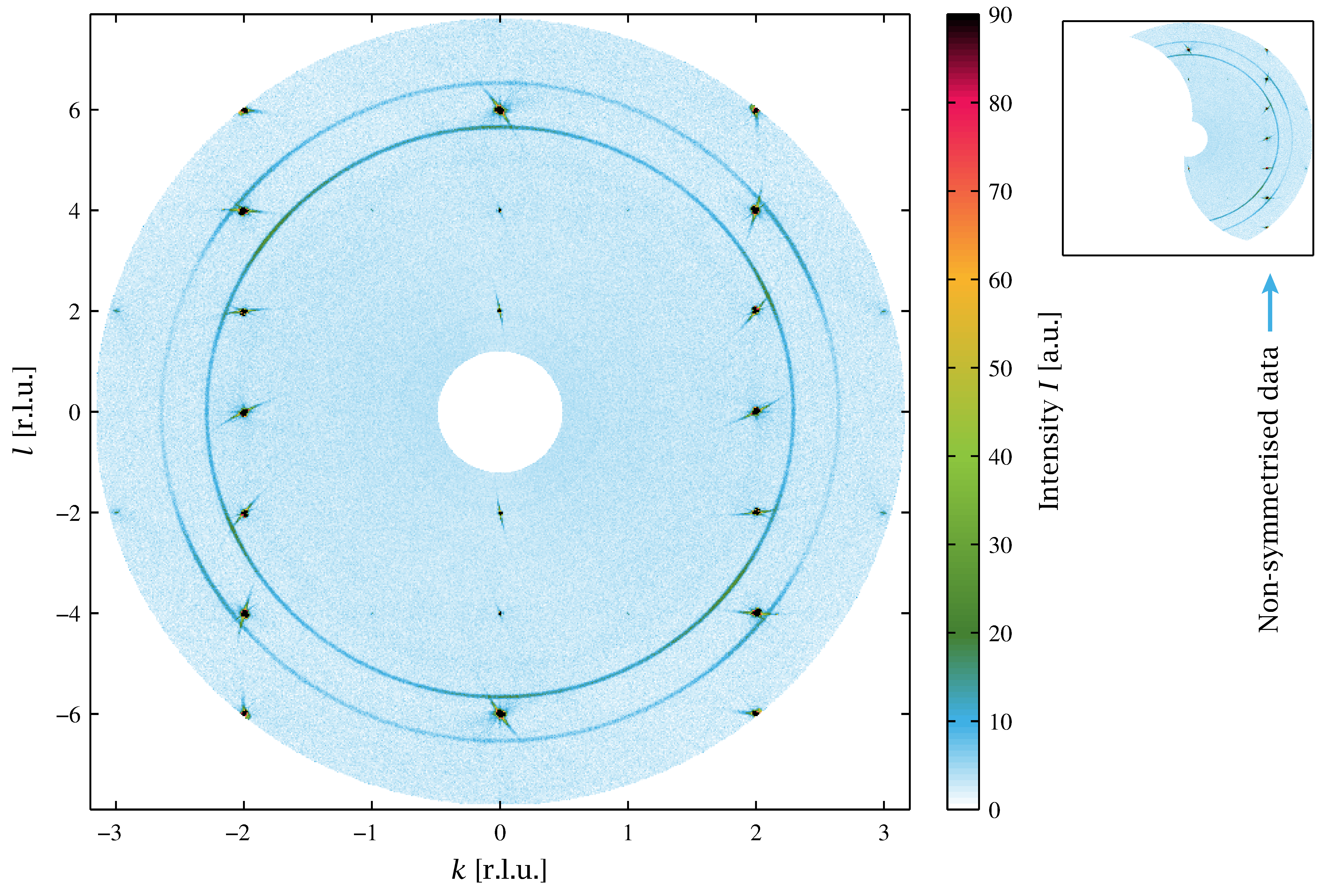
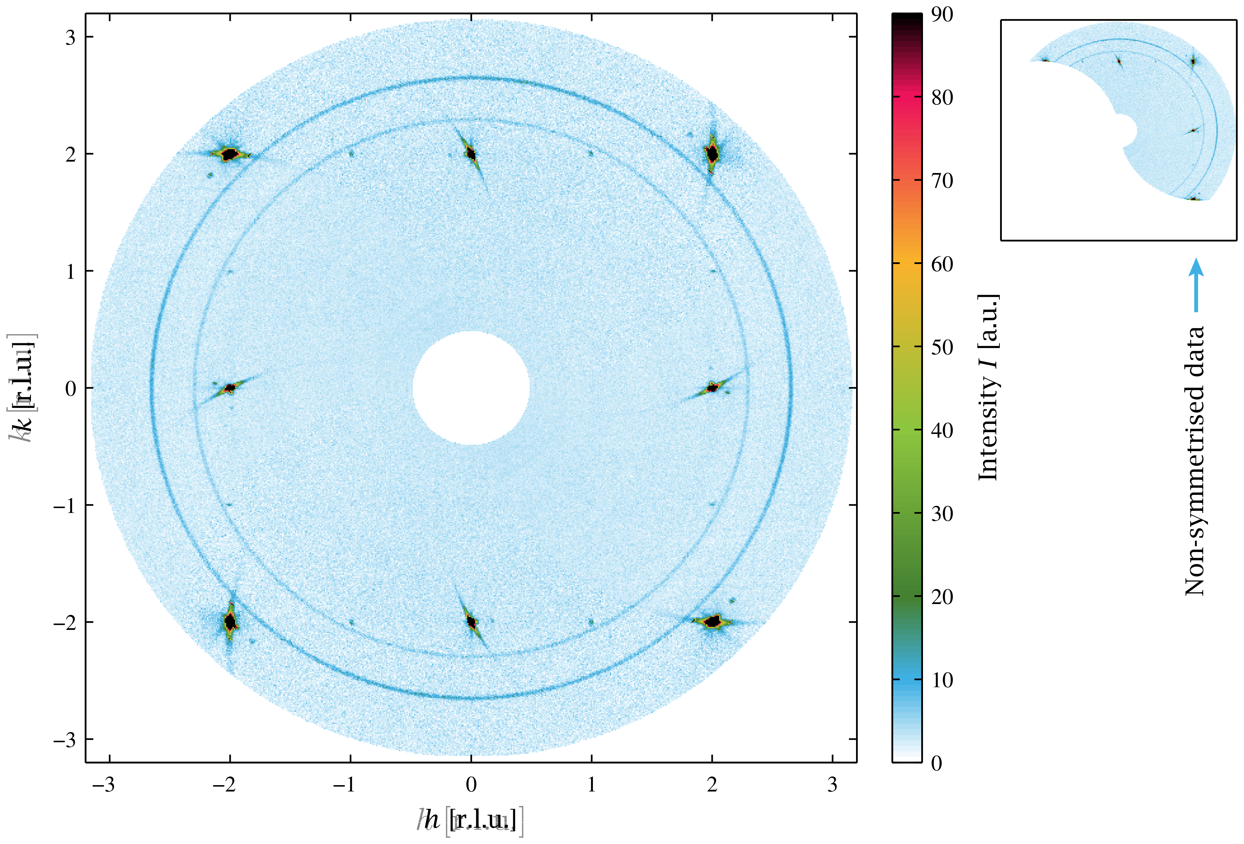
Figur 9.8(a): DMC comparison plots - unwarped (0kl) SXD plane at 290 K. Download links:PNG • SVG (fuld vektor SVG) • PDF (fuld vektor PDF). .
Figur 9.8(b): DMC comparison plots - unwarped (hk0) SXD plane at 290 K. Download links:PNG • SVG (fuld vektor SVG) • PDF (fuld vektor PDF). .
Figur 9.9: Staging - collapsed DMC-thickness data around eight different Bmab peaks. Download links:PNG • SVG • PDF. .
Figur 9.10: Zoomed in look at the 10 K (0kl) non-integrated plane. Download links:PNG • SVG (fuld vektor SVG) • PDF (fuld vektor PDF). .
Figur 9.11: Staging - comparing collapses of DMC-thick. and non-int. maps at 10 K. Download links:PNG • SVG • PDF. .
Figur 9.12: Chains - comparing collapses of DMC-thick. and non-int. maps at 10 K and 290 K. Download links:PNG • SVG • PDF. .
Figur 9.13(a): A look at the (1kl) plane at 10 K. Download links:PNG • SVG (fuld vektor SVG) • PDF (fuld vektor PDF). .
Figur 9.13(b): A look at the (1kl) plane at 290 K. Download links:PNG • SVG (fuld vektor SVG) • PDF (fuld vektor PDF). .
Figur 9.14: SXD animation snapshots - kl planes at 10 K. Download links:PNG • SVG (fuld vektor SVG) • PDF (fuld vektor PDF). .
Figur 9.15: SXD animation snapshots - hk planes at 10 K. Download links:PNG • SVG (fuld vektor SVG) • PDF (fuld vektor PDF). .
Laboratorie-røntgen-illustrationer og dataplots (kapitel 10)
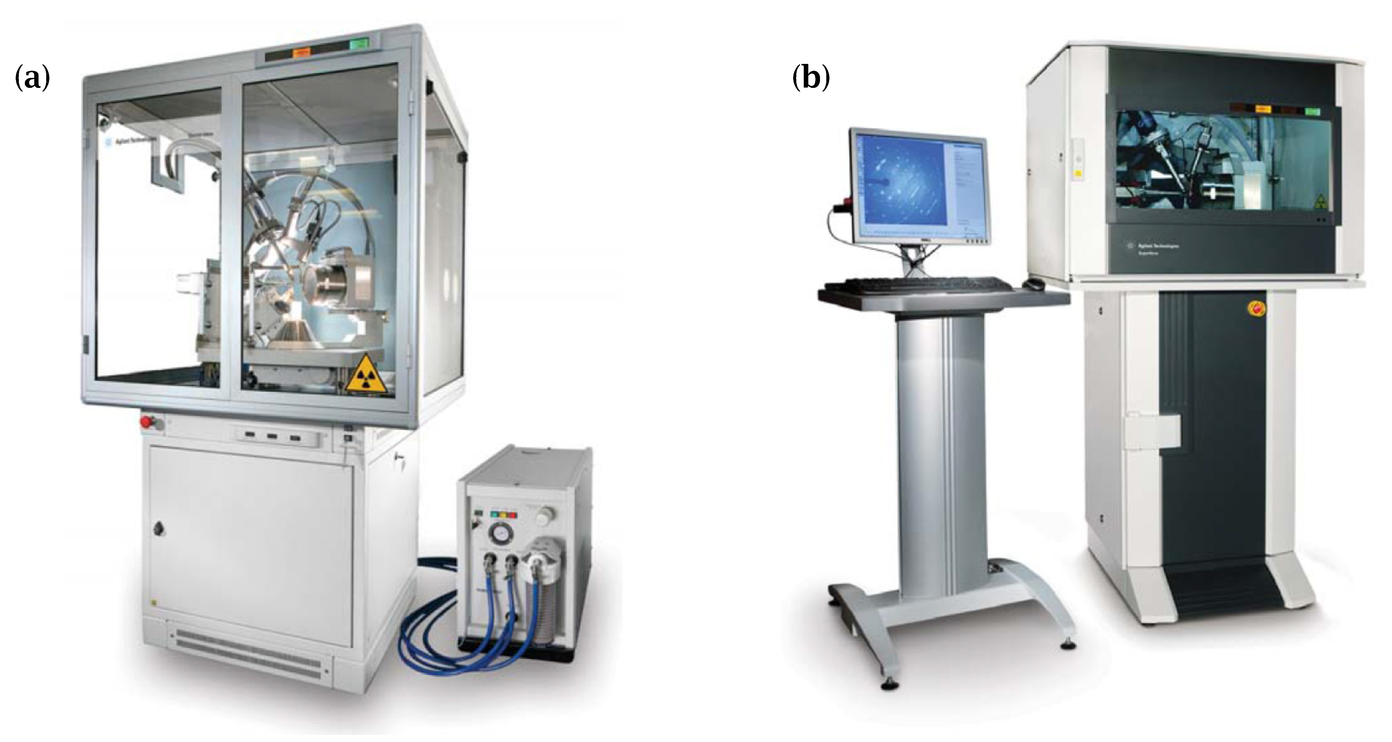
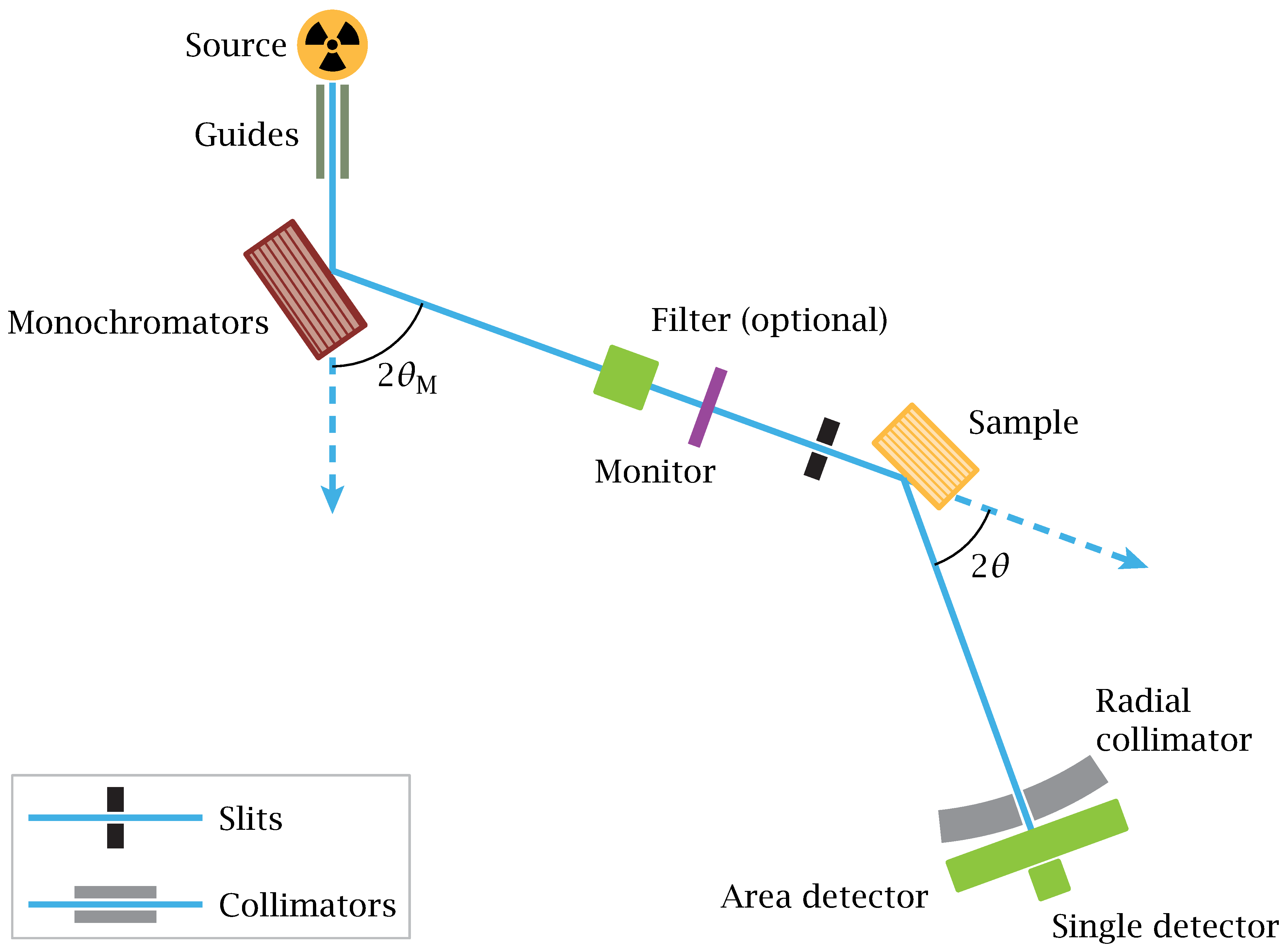
Figur 10.1: The Gemini and SuperNova instruments. Download links:PNG • SVG • PDF. .
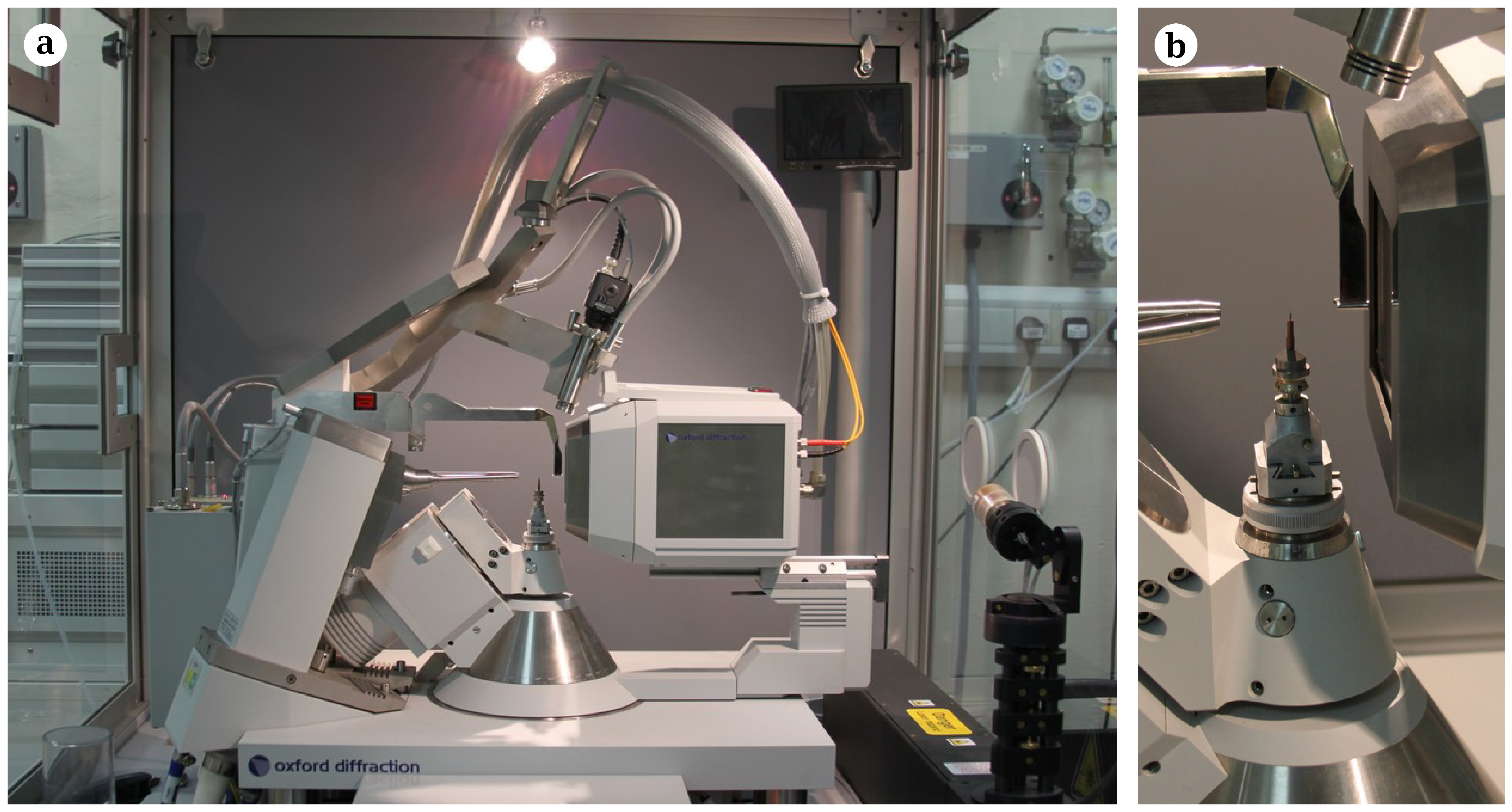
Figur 10.2: Photos of the Gemini laboratory X-ray instrument setup. Download links:PNG • αPNG • SVG • PDF. .
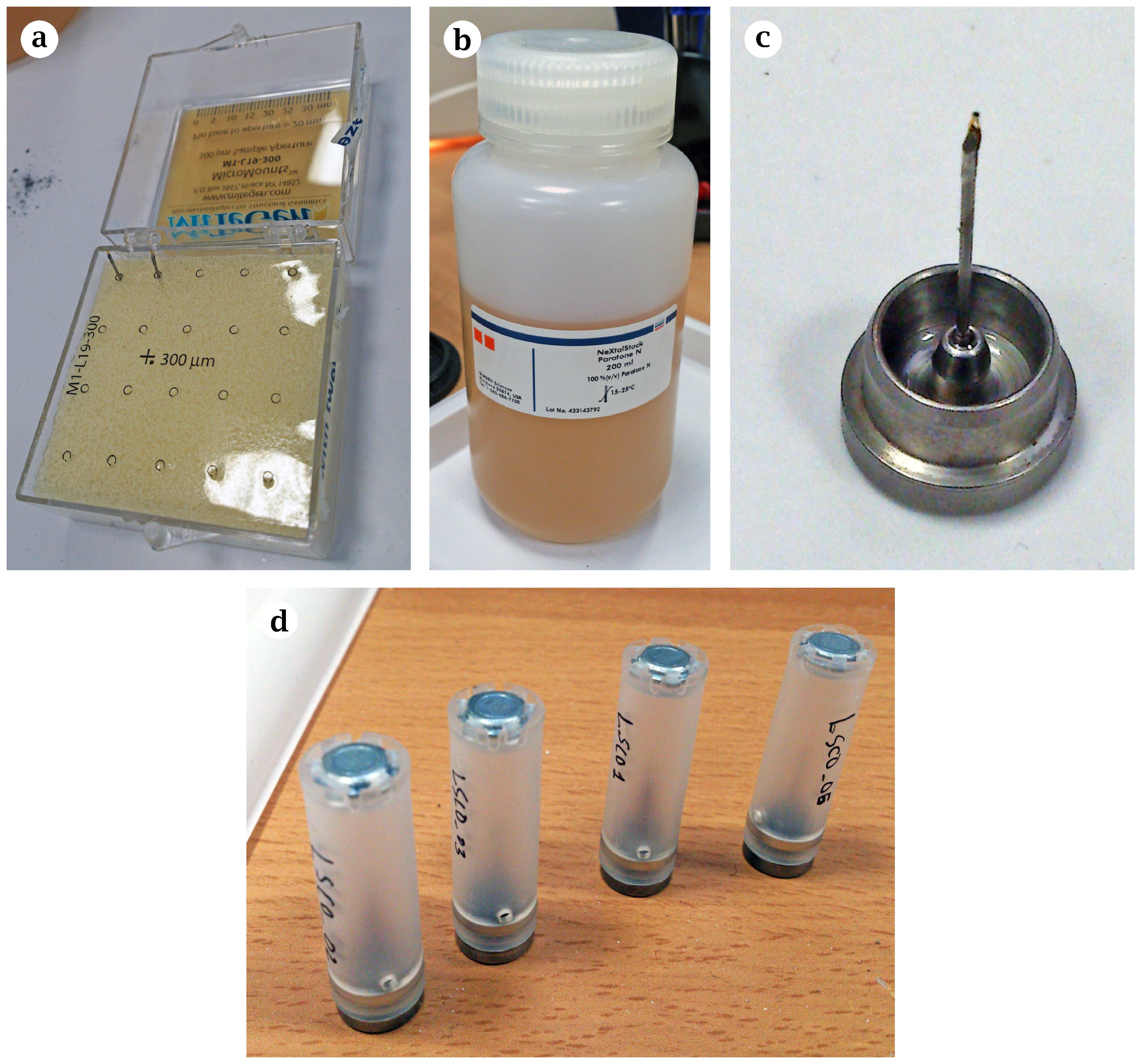
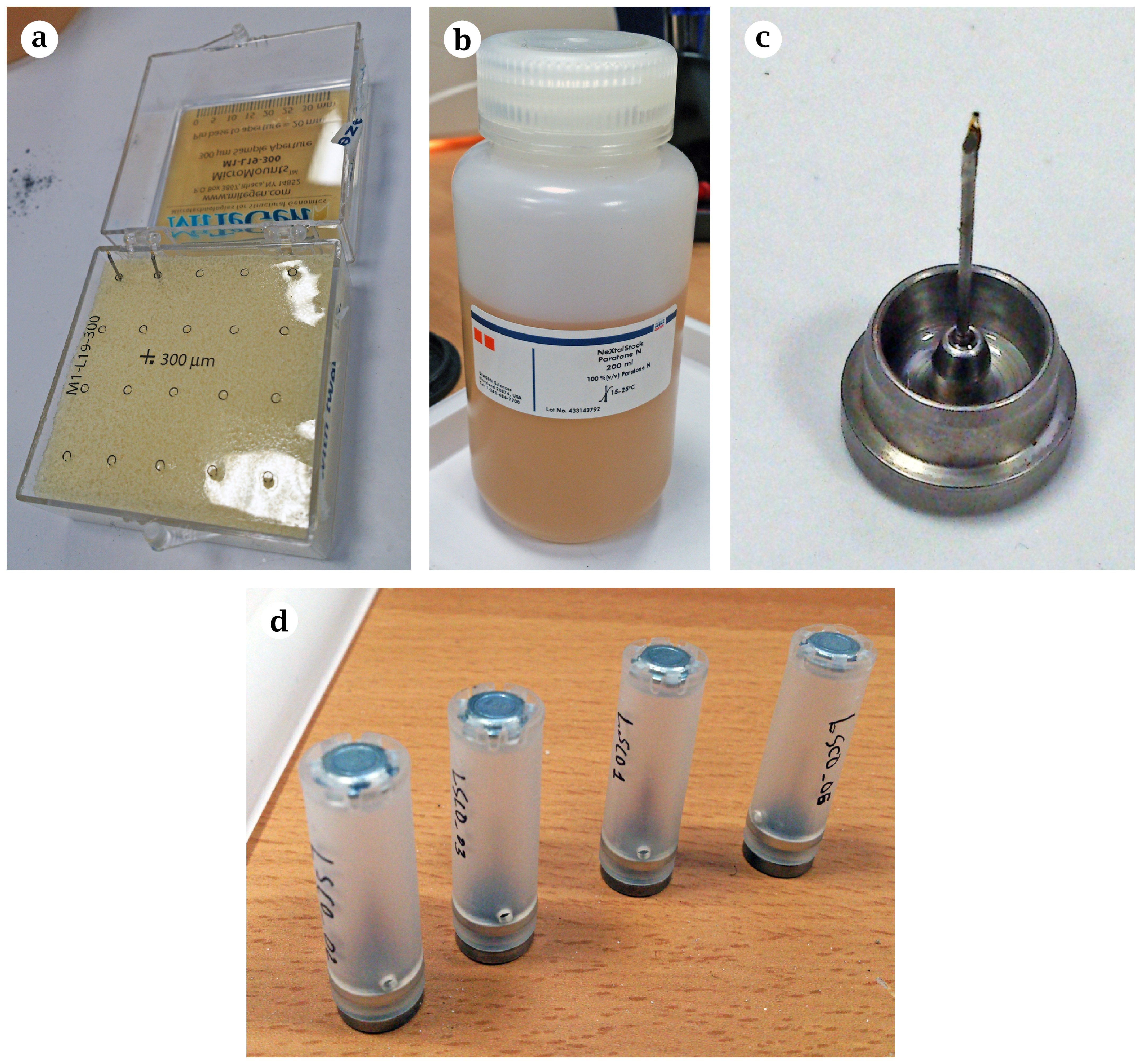
Figur 10.3: Mounting of the samples to kapton loops. Download links:PNG • αPNG • SVG • PDF. .
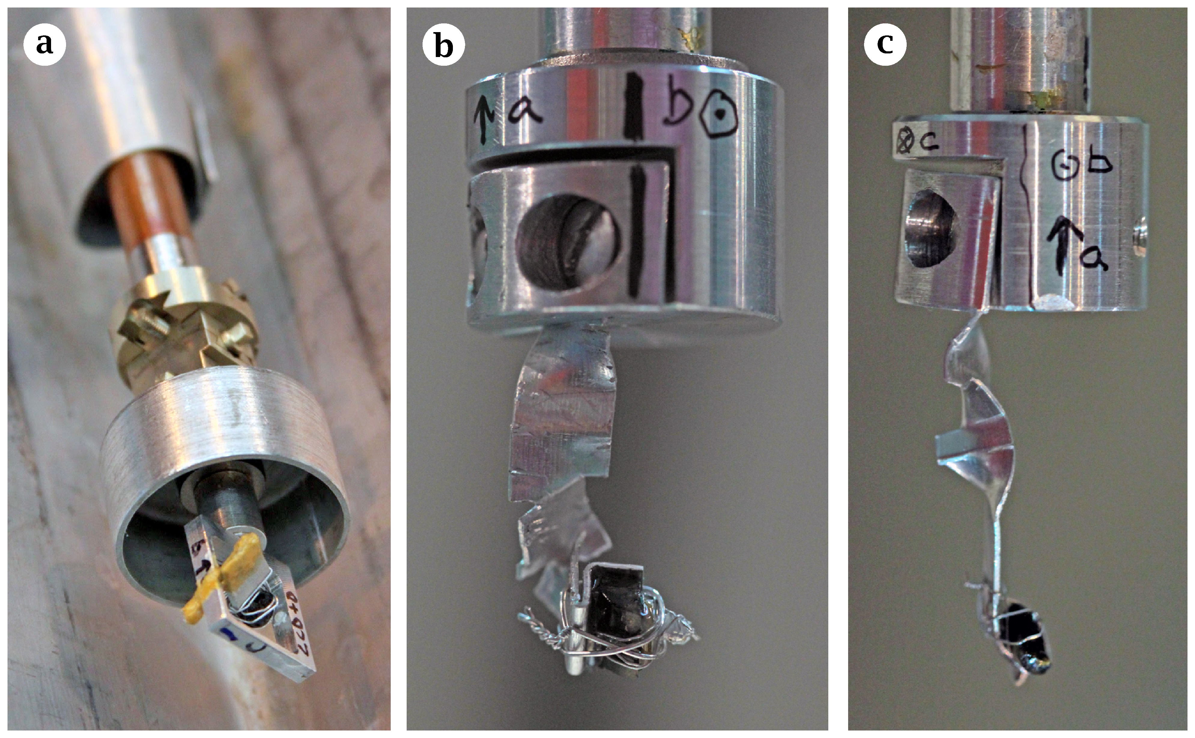
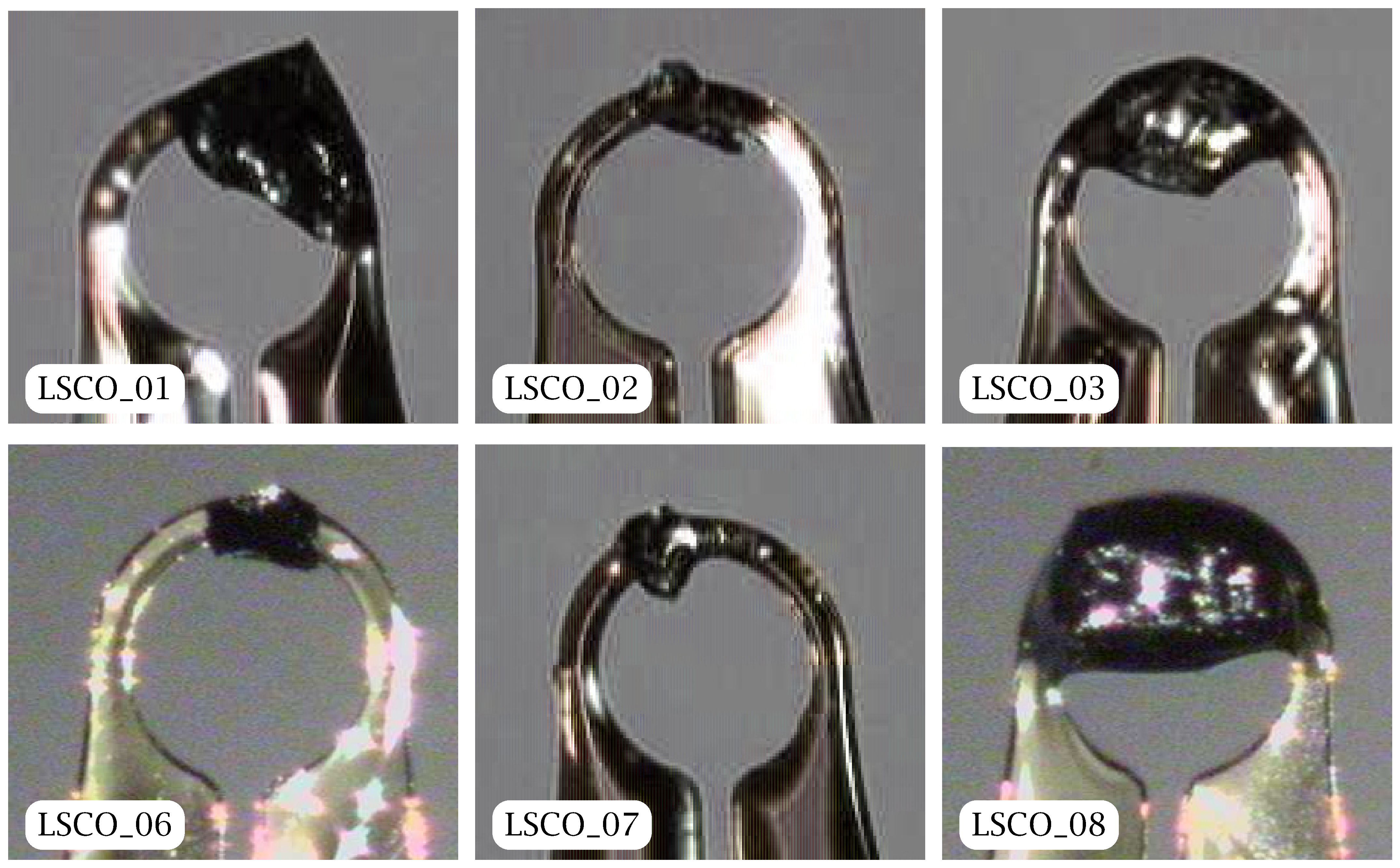
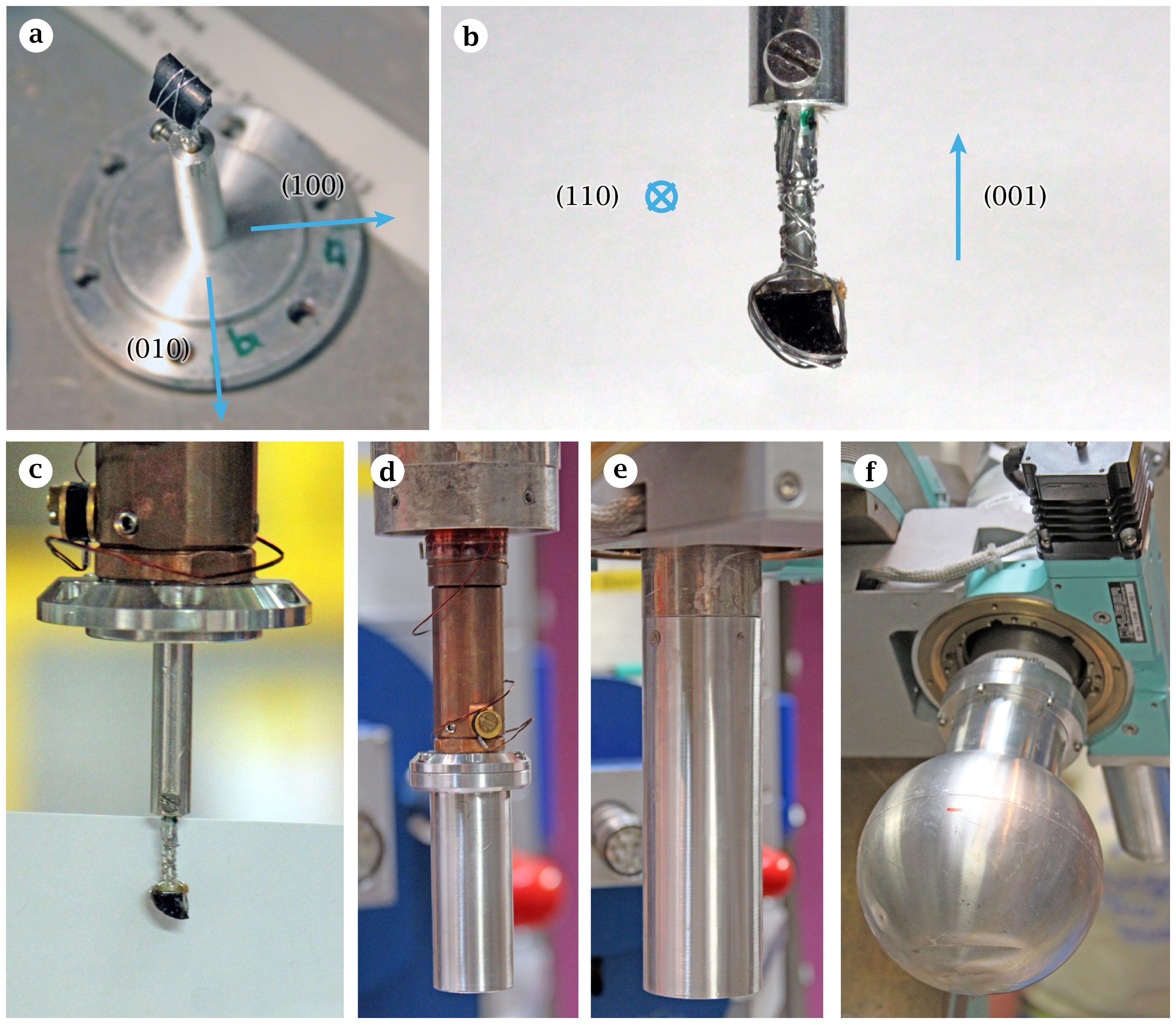
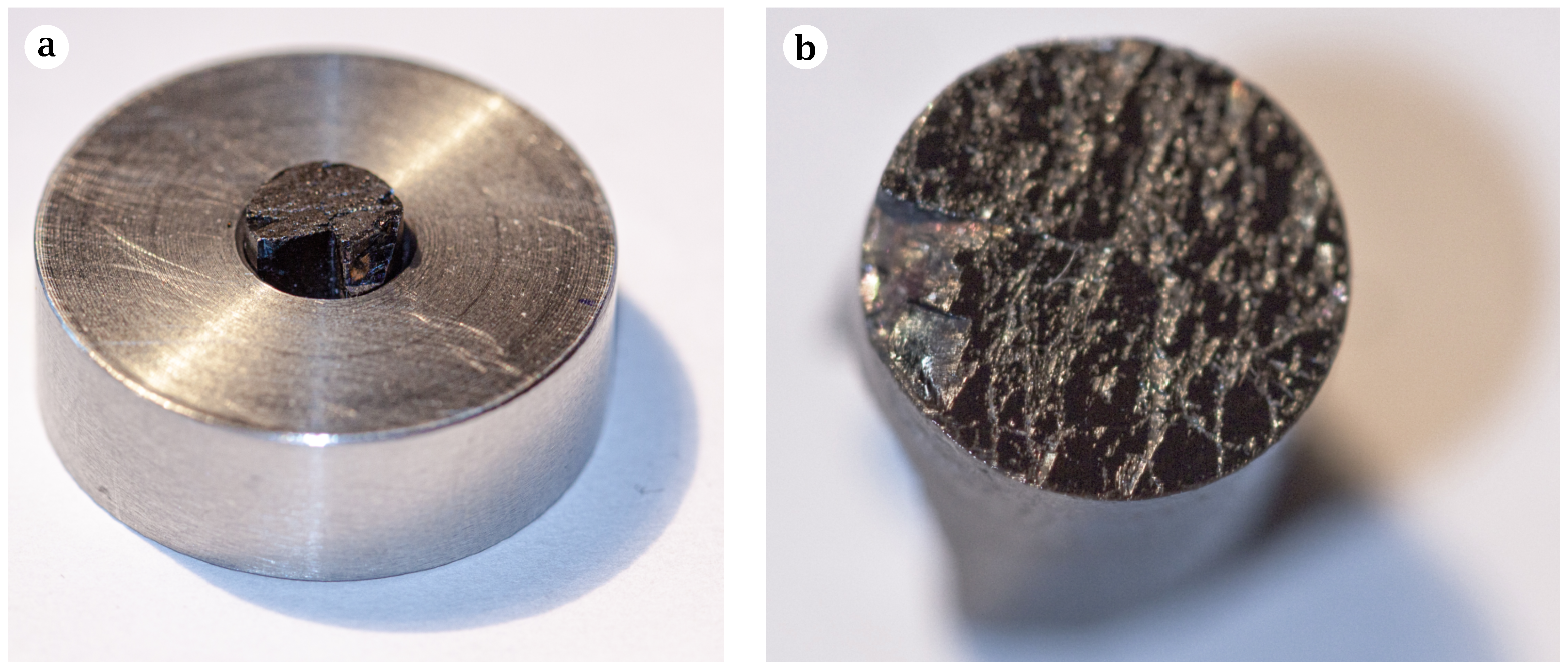
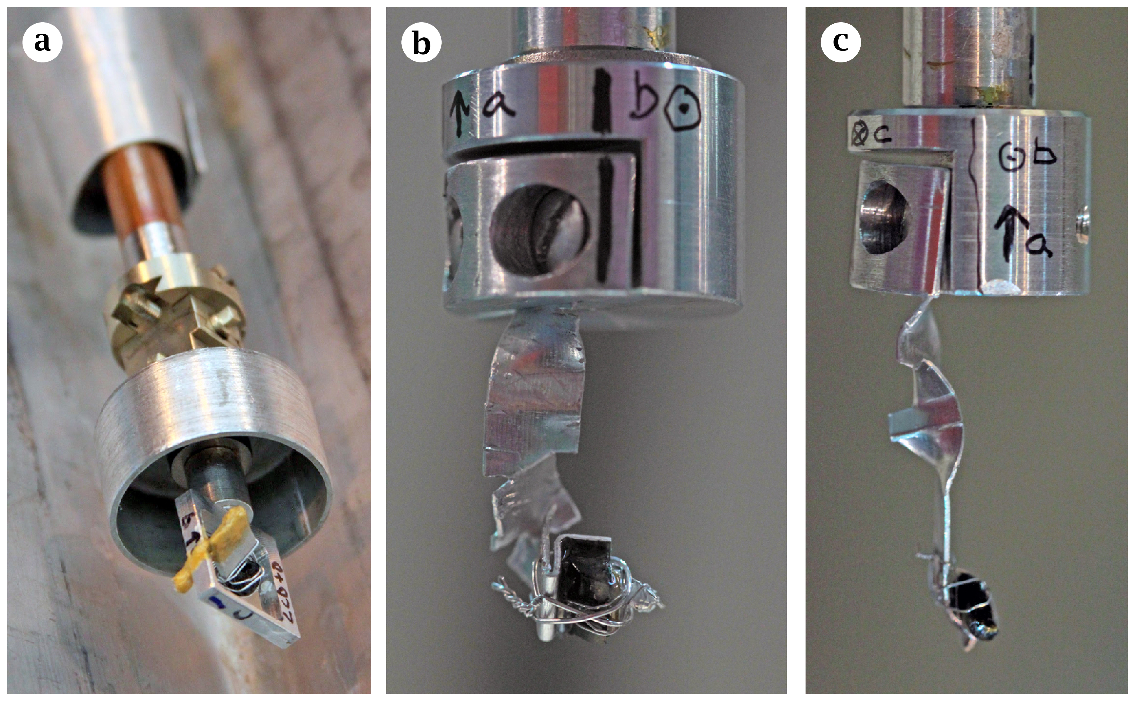
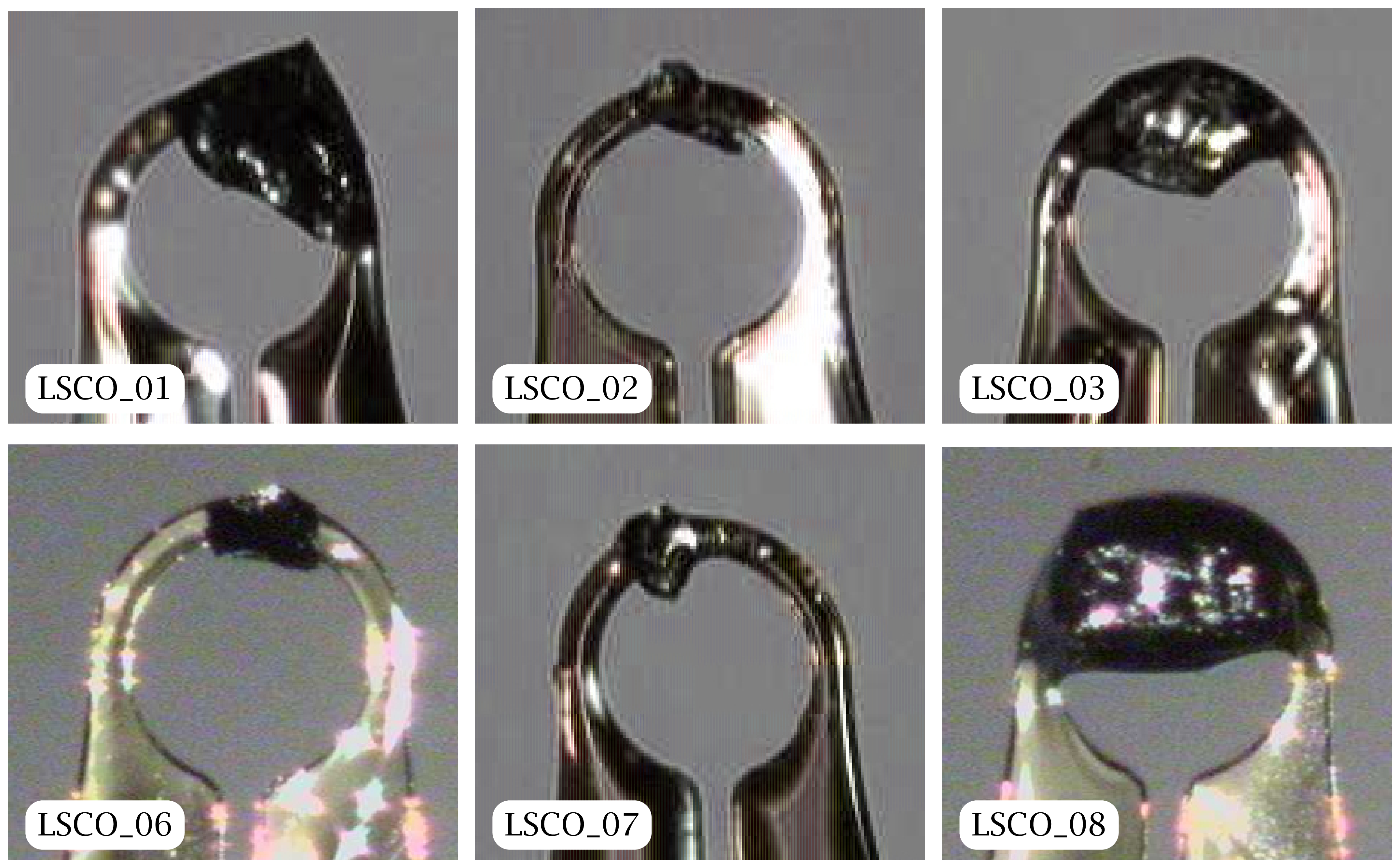
Figur 10.4: Close-up photos of the samples measured on the laboratory X-ray instruments. Download links:PNG • αPNG • SVG • PDF. .
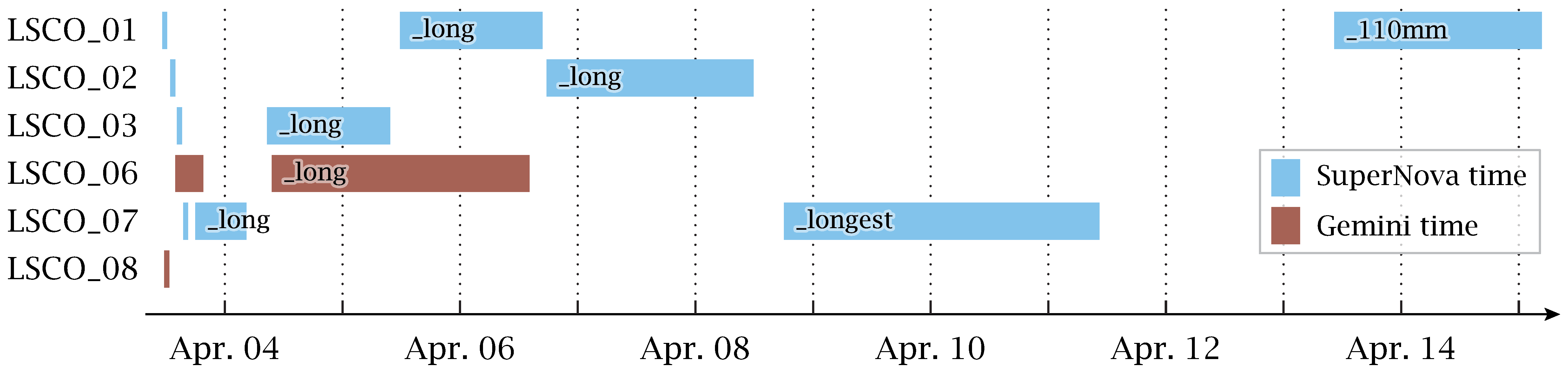
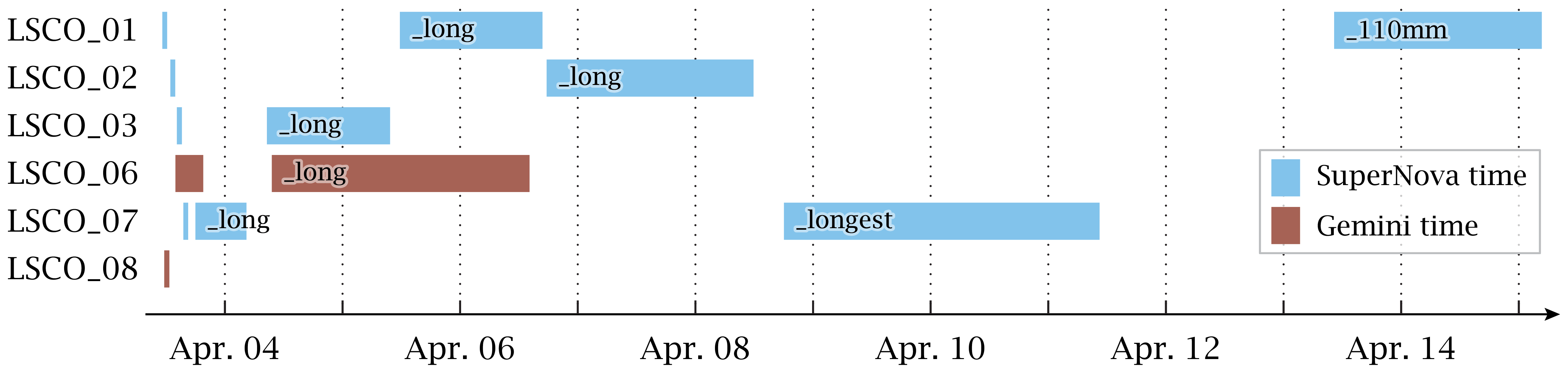
Figur 10.5: Timeline of the laboratory X-ray measurements on the six main samples. Download links:PNG • αPNG • SVG • PDF. .
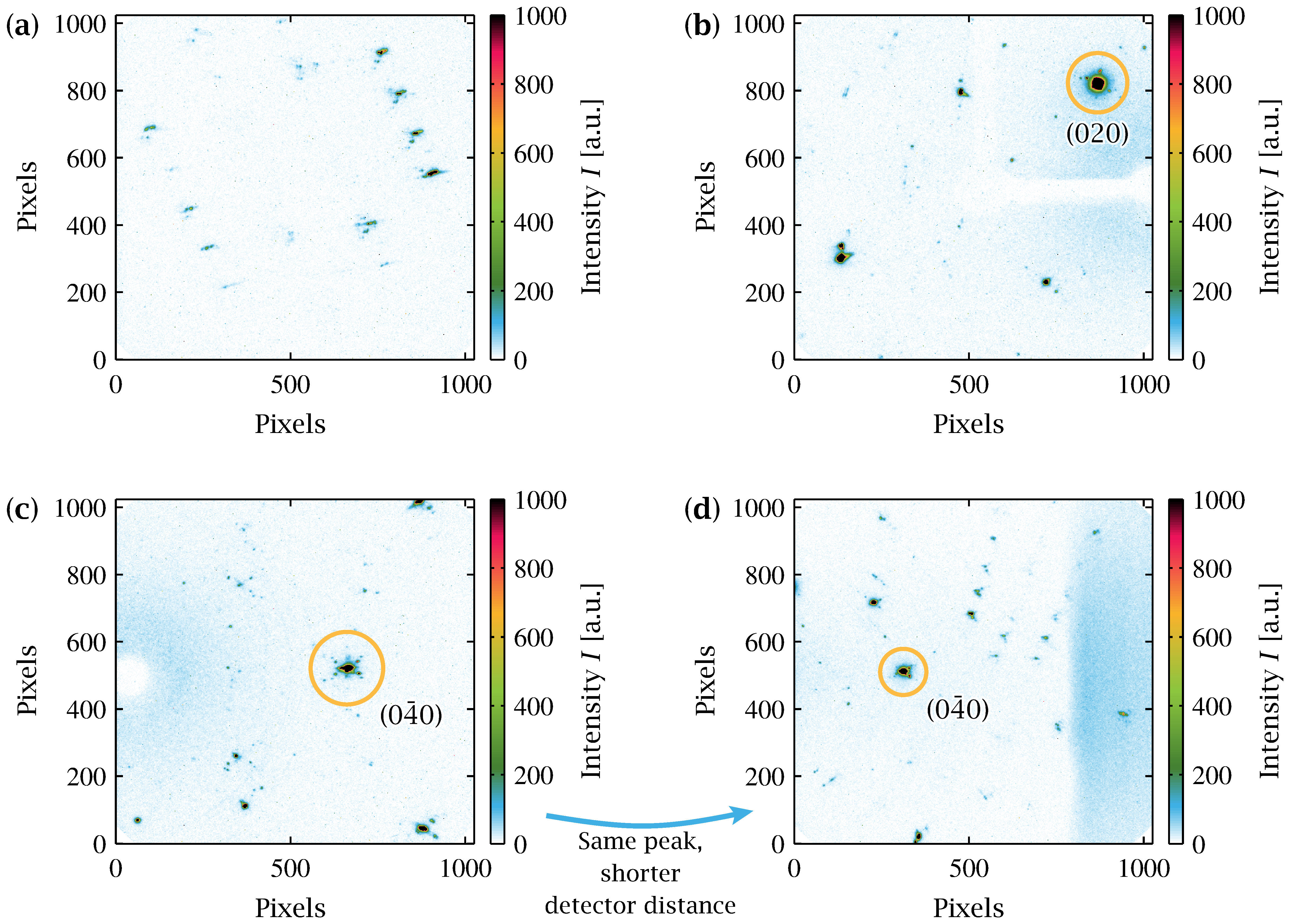
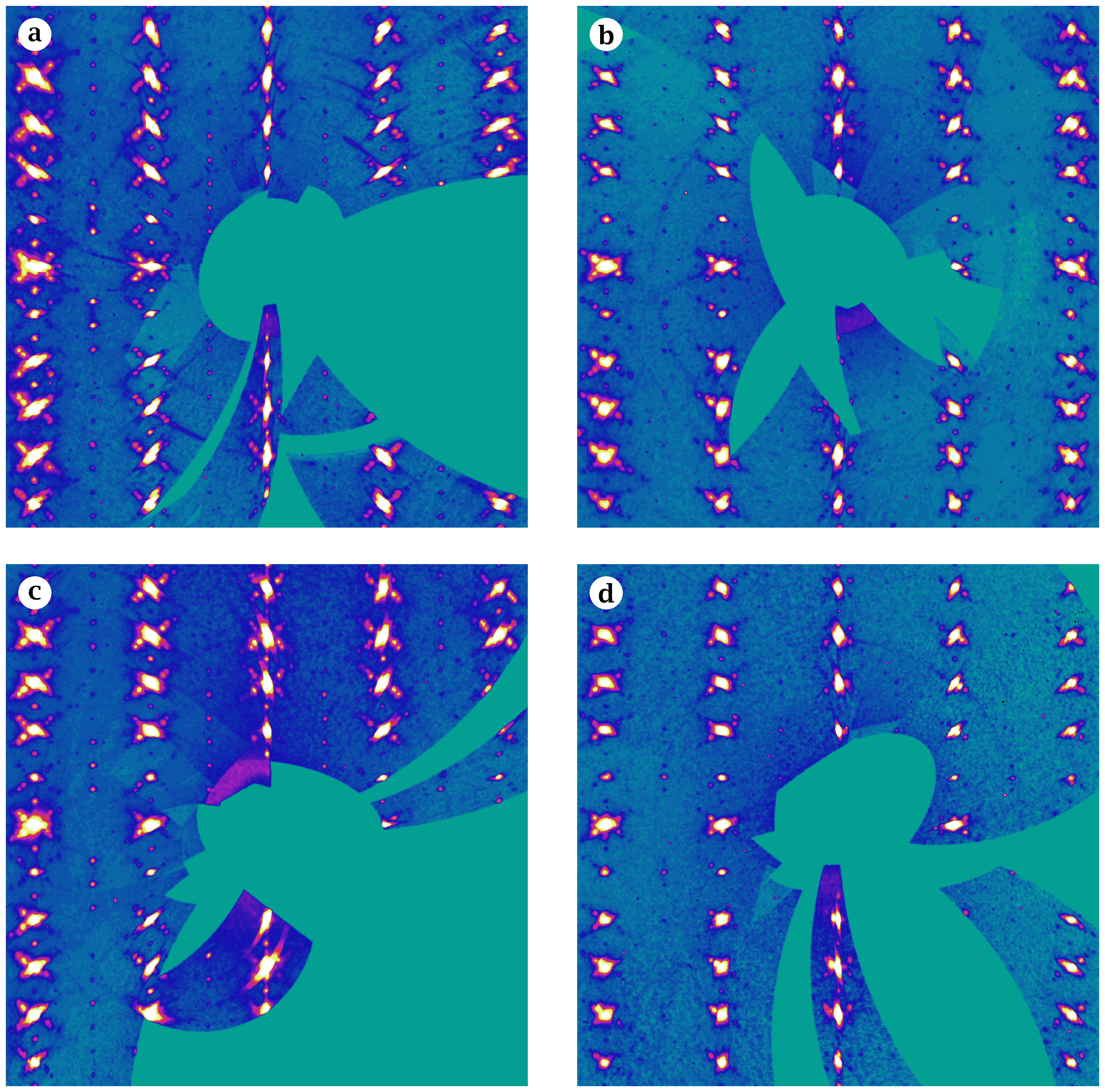
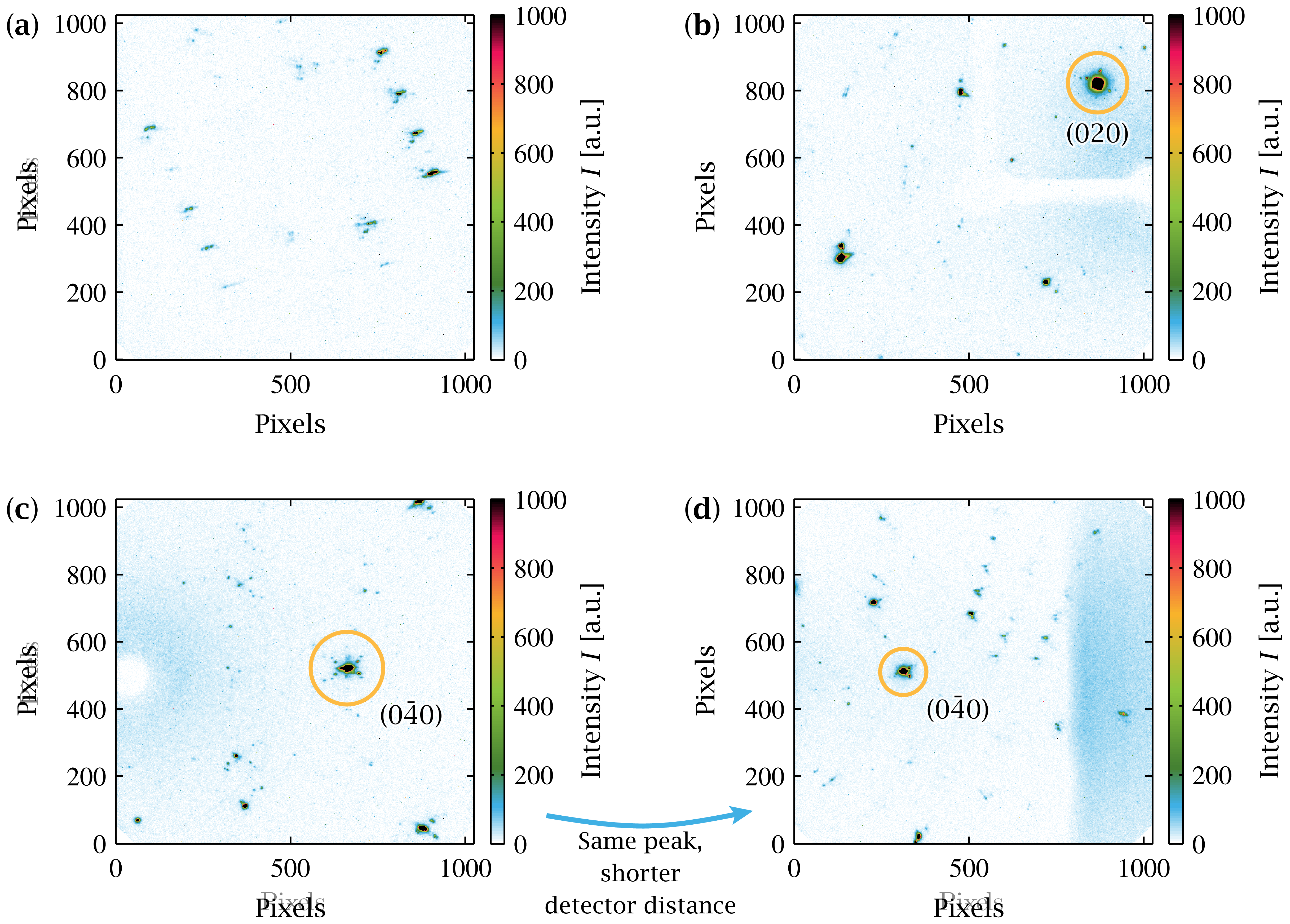
Figur 10.6: Examples of raw laboratory X-ray frames. Download links:PNG • αPNG • SVG (fuld vektor SVG) • PDF (fuld vektor PDF). .
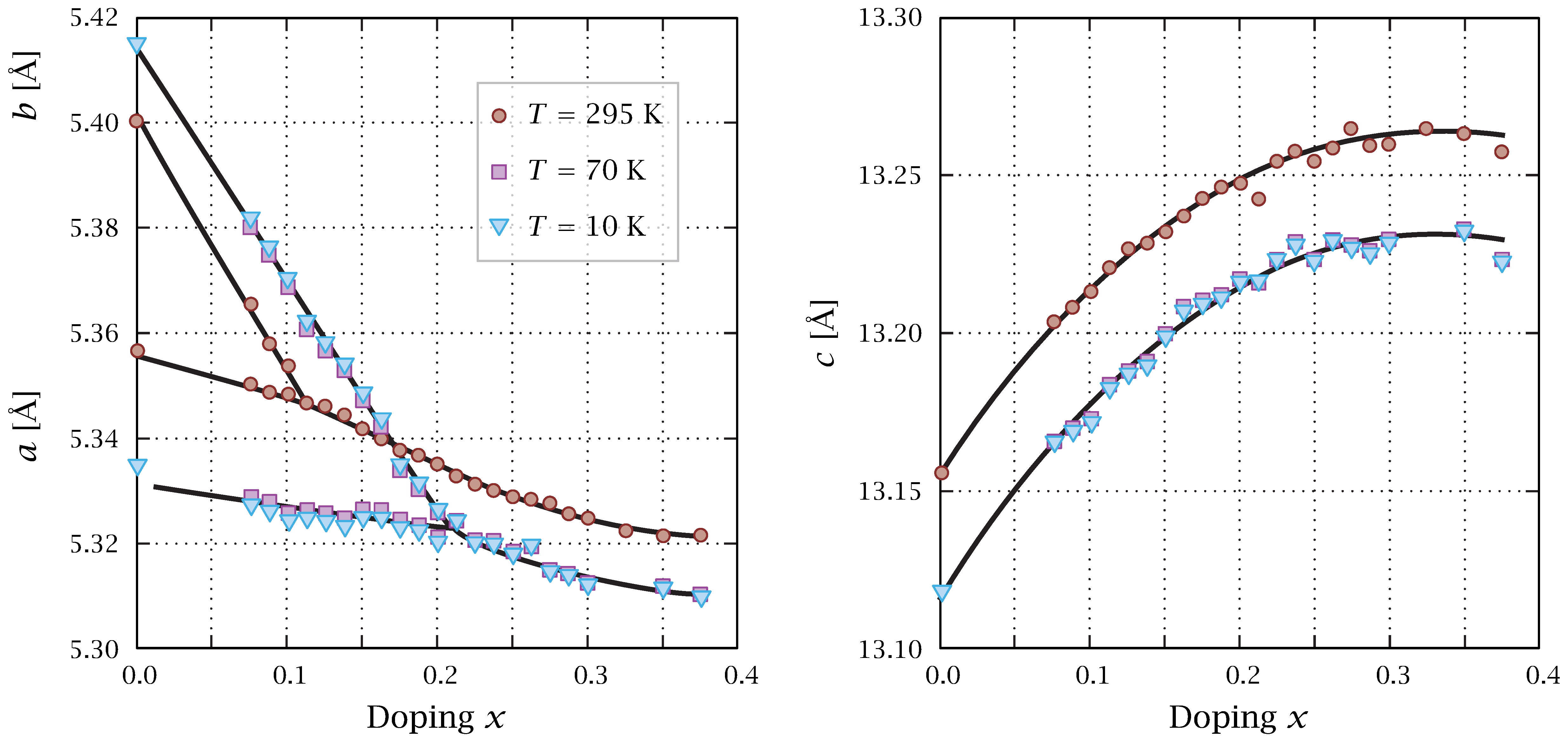
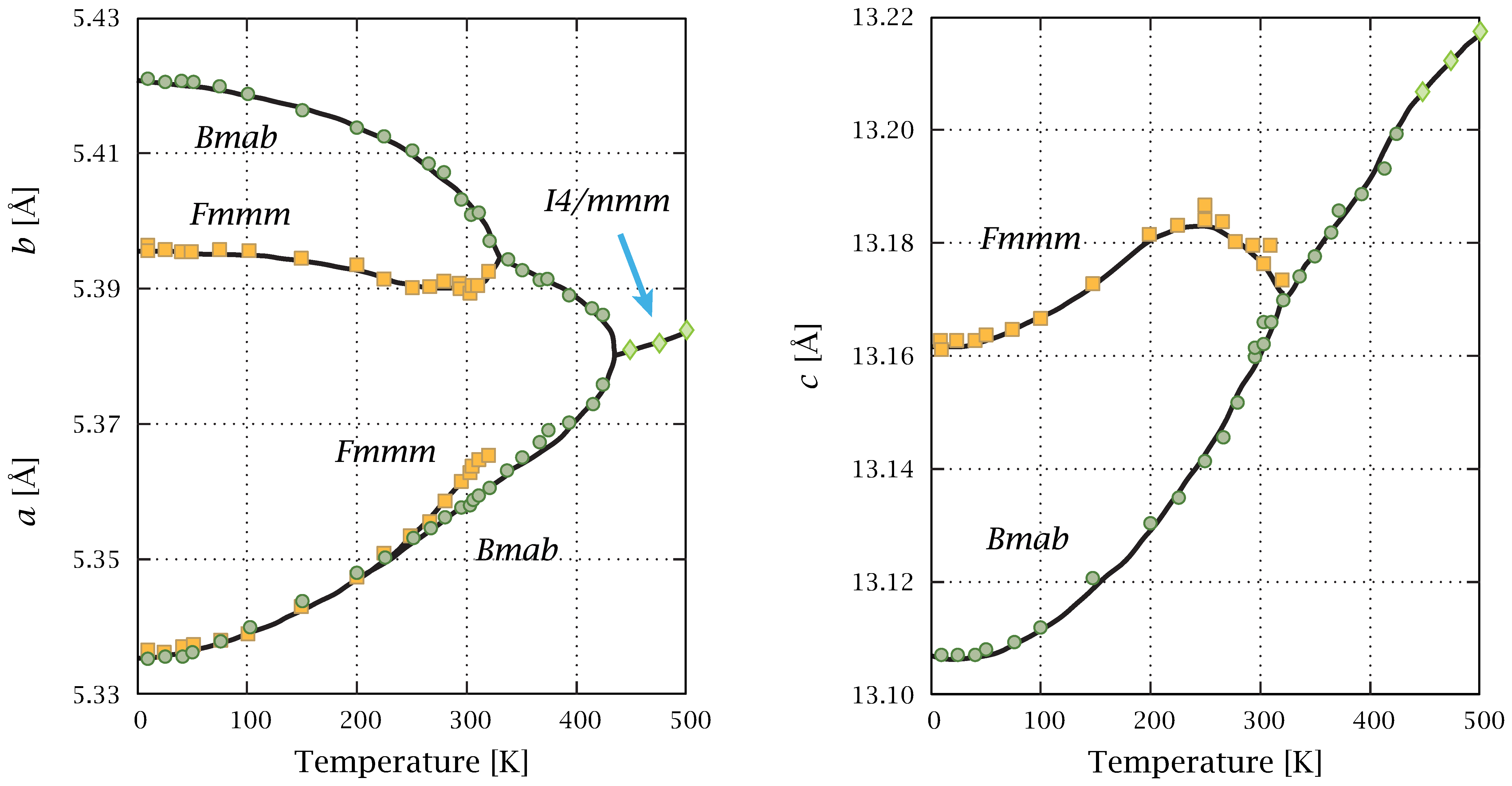
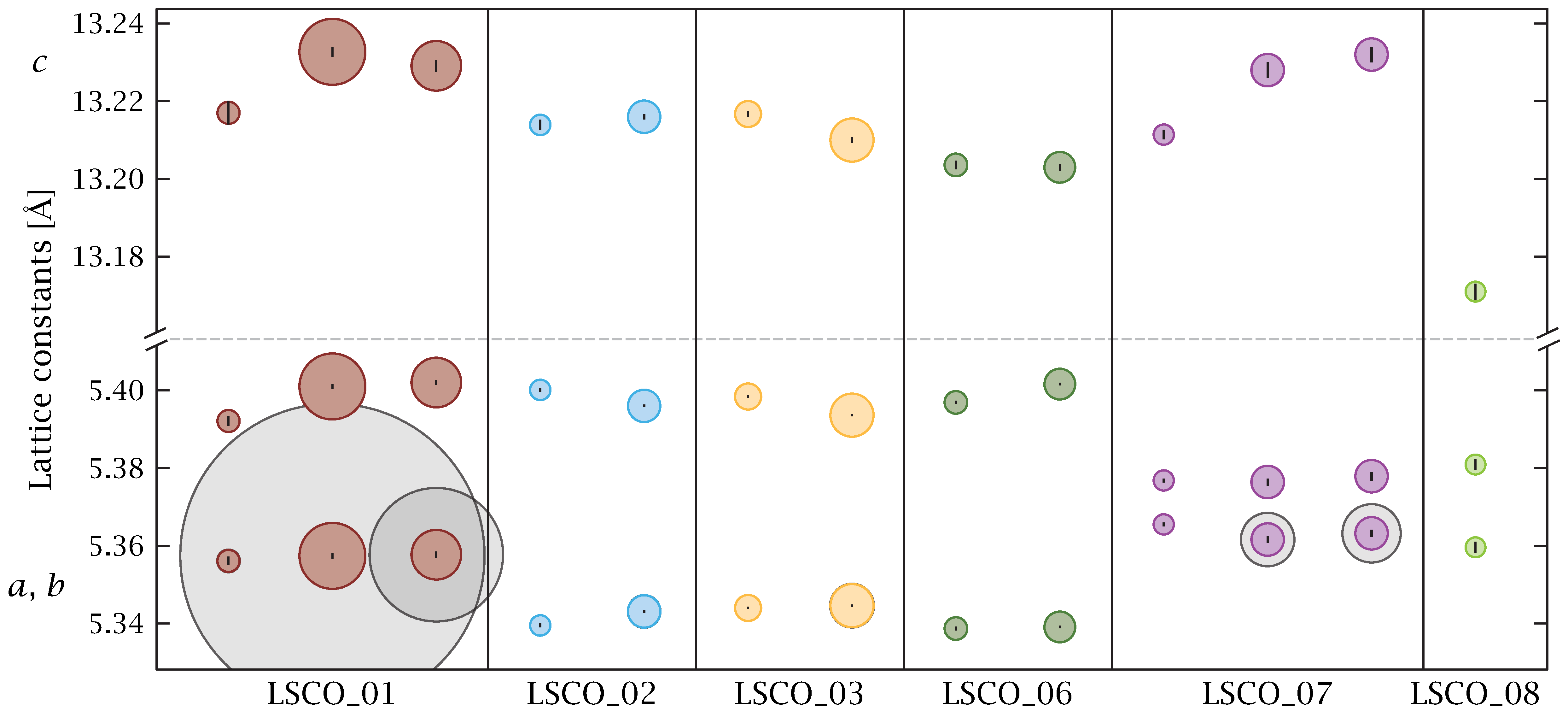
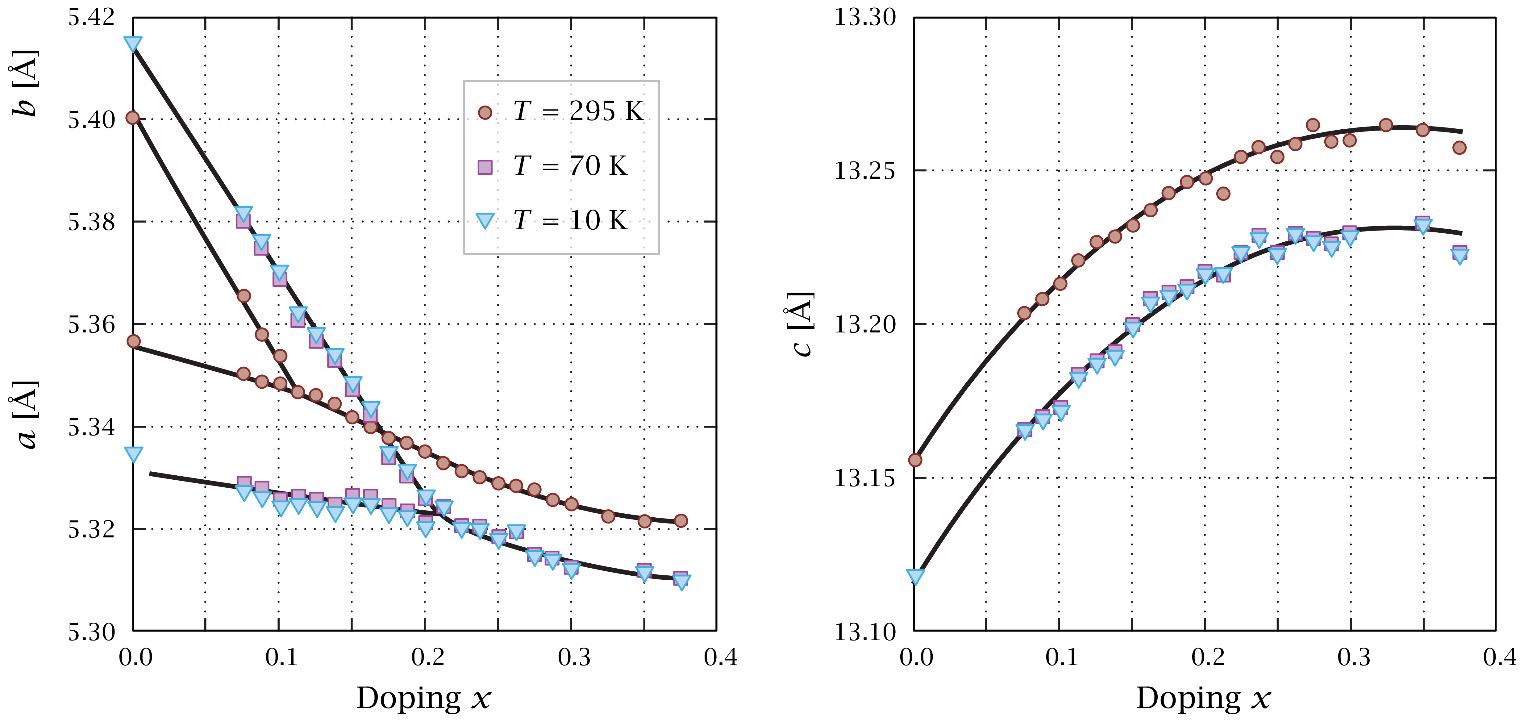
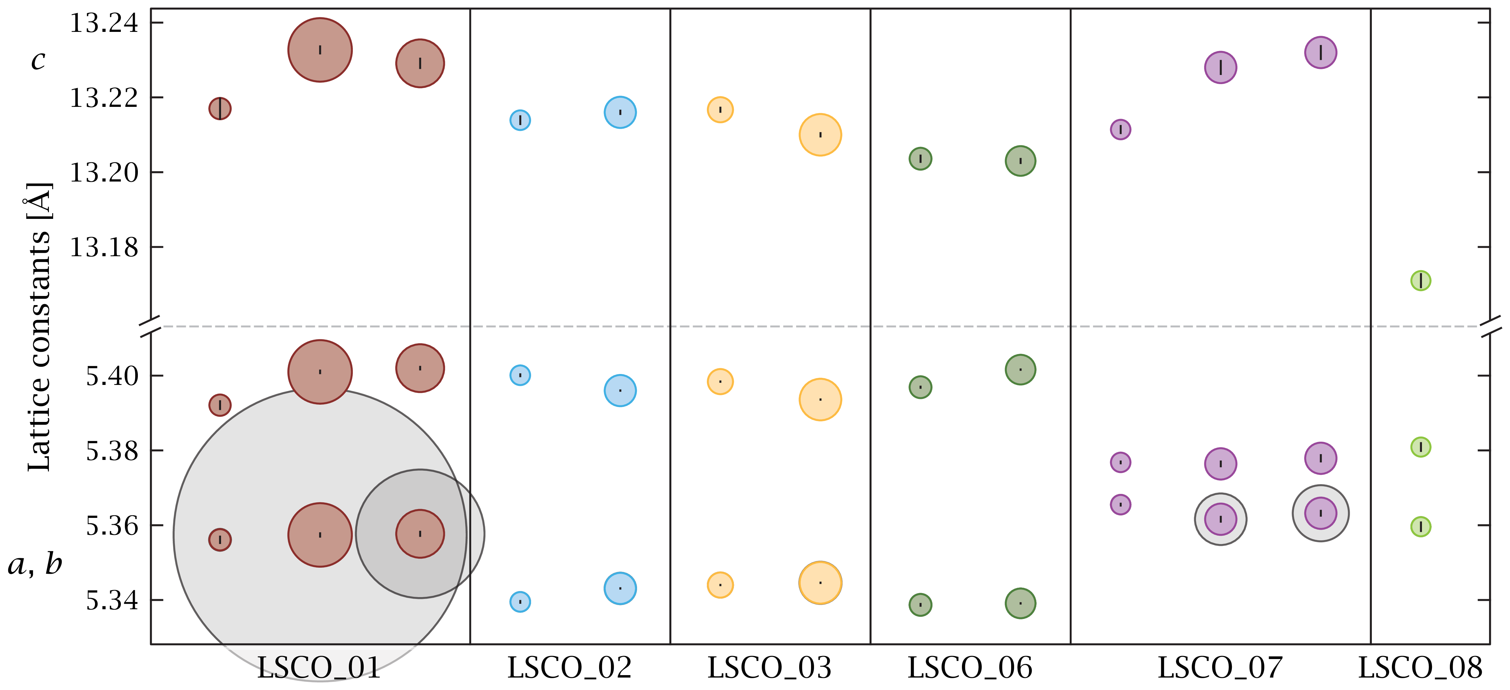
Figur 10.7: Overview of lattice constants found in X-ray source measurements. Download links:PNG • αPNG • SVG • PDF. .
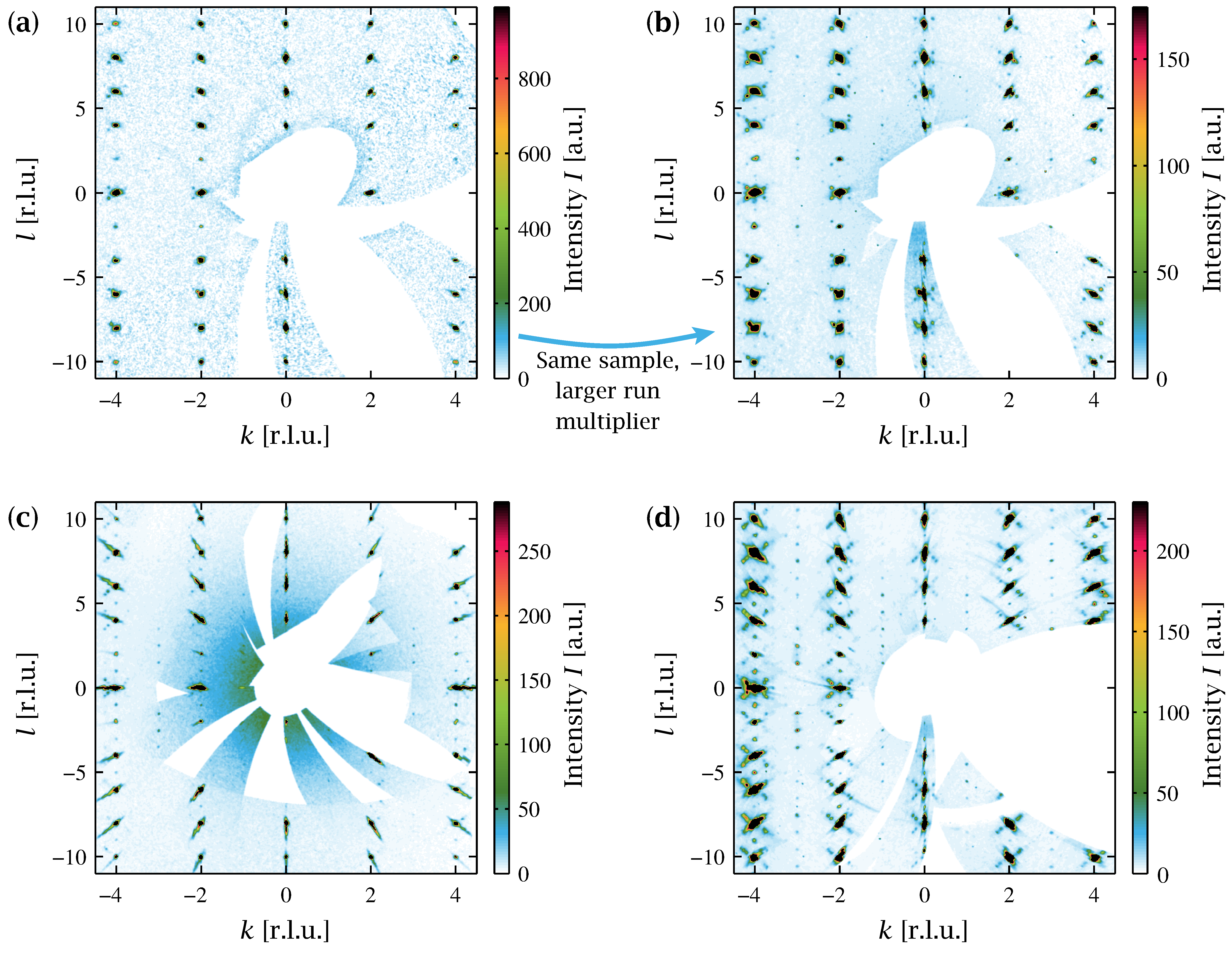
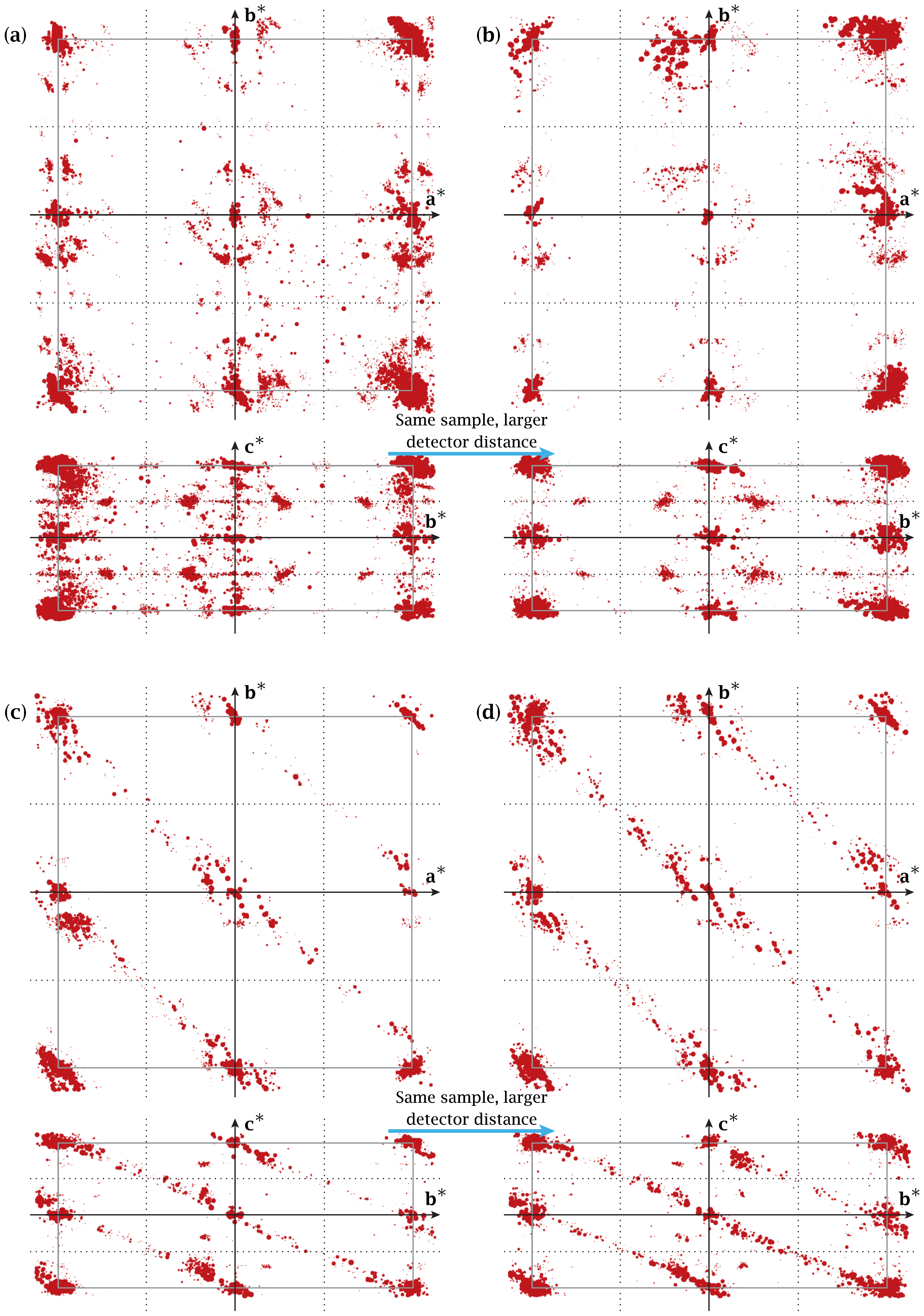
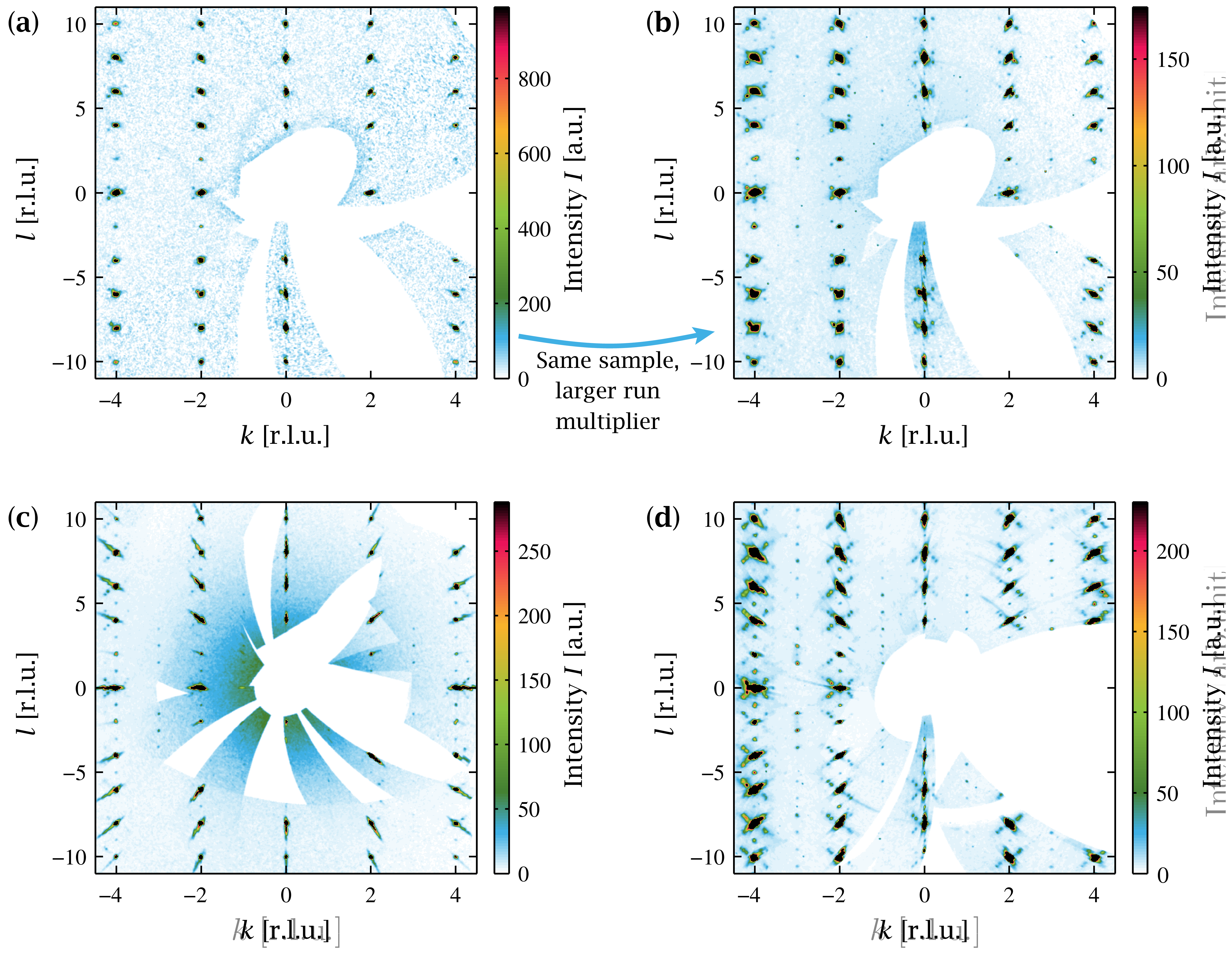
Figur 10.8: Unwarped (0kl) planes for some of the main data sets. Download links:PNG • αPNG • SVG (fuld vektor SVG) • PDF (fuld vektor PDF). .
Figur 10.9: Unwarped (0kl) plane of the LSCO_01_long scan (non-symmetrised and symmetrised). Download links:PNG • αPNG • SVG • PDF. .
Figur 10.10: Unwarped (hk0) plane of the LSCO_01_long scan (non-symmetrised and symmetrised). Download links:PNG • αPNG • SVG • PDF. .
Figur 10.11: Examples of Ewald3D views from the CrysAlis software. Download links:PNG • αPNG • SVG • PDF. .
Figur 10.12: Unwarped kl planes at varied h - showing volume for LSCO_01_long scan. Download links:PNG • αPNG • SVG • PDF. .
Figur 10.13: Unwarped (0kl) and (hk0) planes of the LSCO_01_long scan in full view. Download links:PNG • αPNG • SVG • PDF. .
Figur 10.14: Examples of unwarped (0kl) planes exported directly from CrysAlis. Download links:PNG • αPNG • SVG • PDF. .
Figur 10.15: Unwarped (0kl) planes for LSCO_01 and LSCO_07 - zoom around (0,-3,2). Download links:PNG • αPNG • SVG • PDF. .
Figur 10.16: Unwarped (0kl) planes for LSCO_01 and LSCO_07 - zoom around (0,-2,4). Download links:PNG • αPNG • SVG • PDF. .
Figur 10.17: Unwarped (0kl) planes for LSCO_01 and LSCO_07 - zoom around (0,0,-6). Download links:PNG • αPNG • SVG • PDF. .
Figur 10.18: Unwarped (hk0), (hk1), (hk2), and (hk3) planes for two samples. Download links:PNG • αPNG • SVG • PDF. .
Figur 10.19: DMC comparison plots - for the LSCO_01_long scan. Download links:PNG • αPNG • SVG • PDF. .
TriCS-illustrationer og dataplots (kapitel 11)
Figur 11.1: Overview sketch of the TriCS instrument. Download links:PNG • αPNG • SVG • PDF. .
Figur 11.2: A close-up of the TriCS instrument. Download links:PNG • SVG • PDF. .
Figur 11.3: The La(1.94)Sr(0.06)CuO(4+y) sample measured on TriCS. Download links:PNG • αPNG • SVG • PDF. .
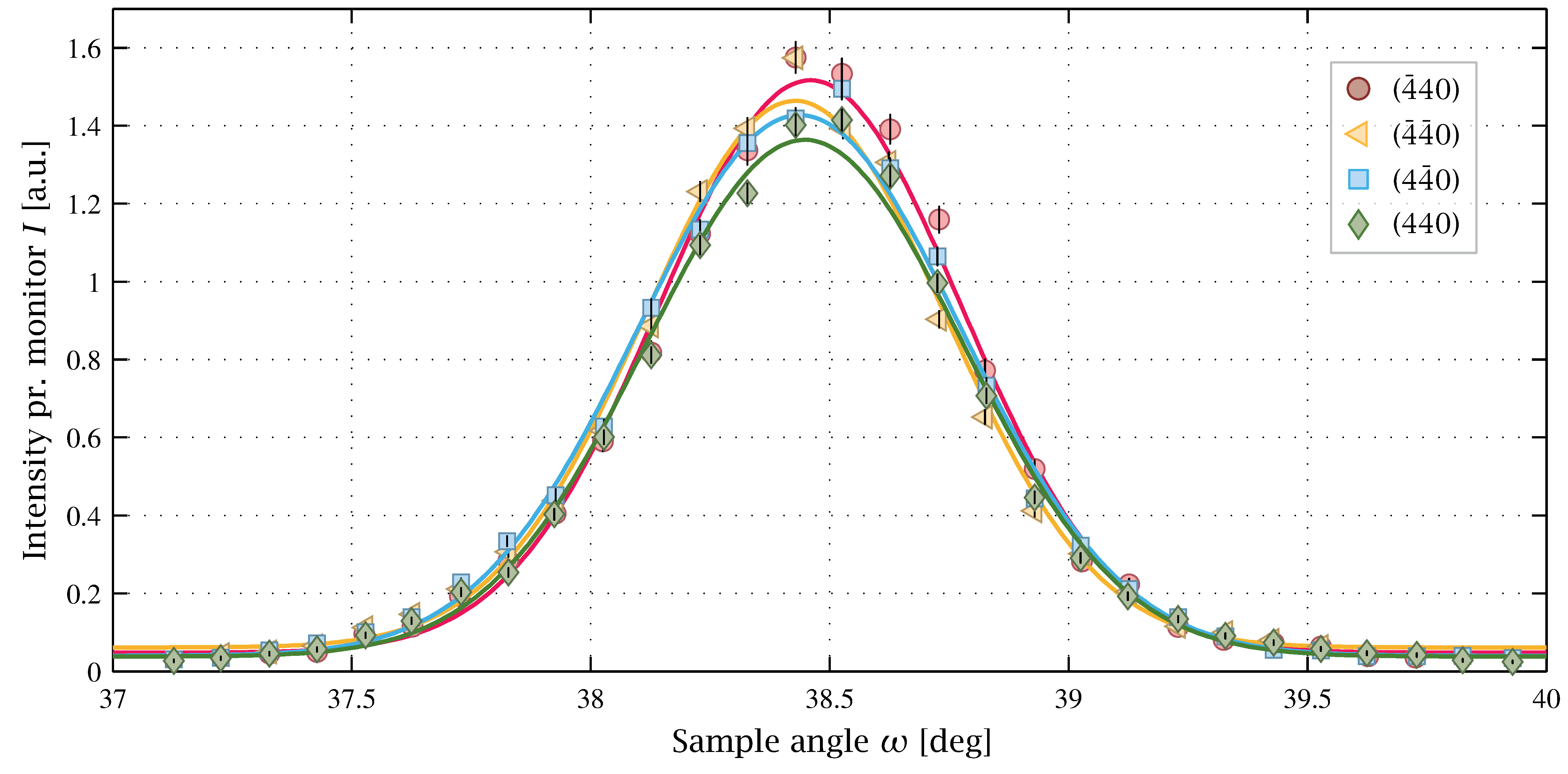
Figur 11.4: The (±4, ±4, 0) peaks measured at room temperature. Download links:PNG • SVG • PDF. .
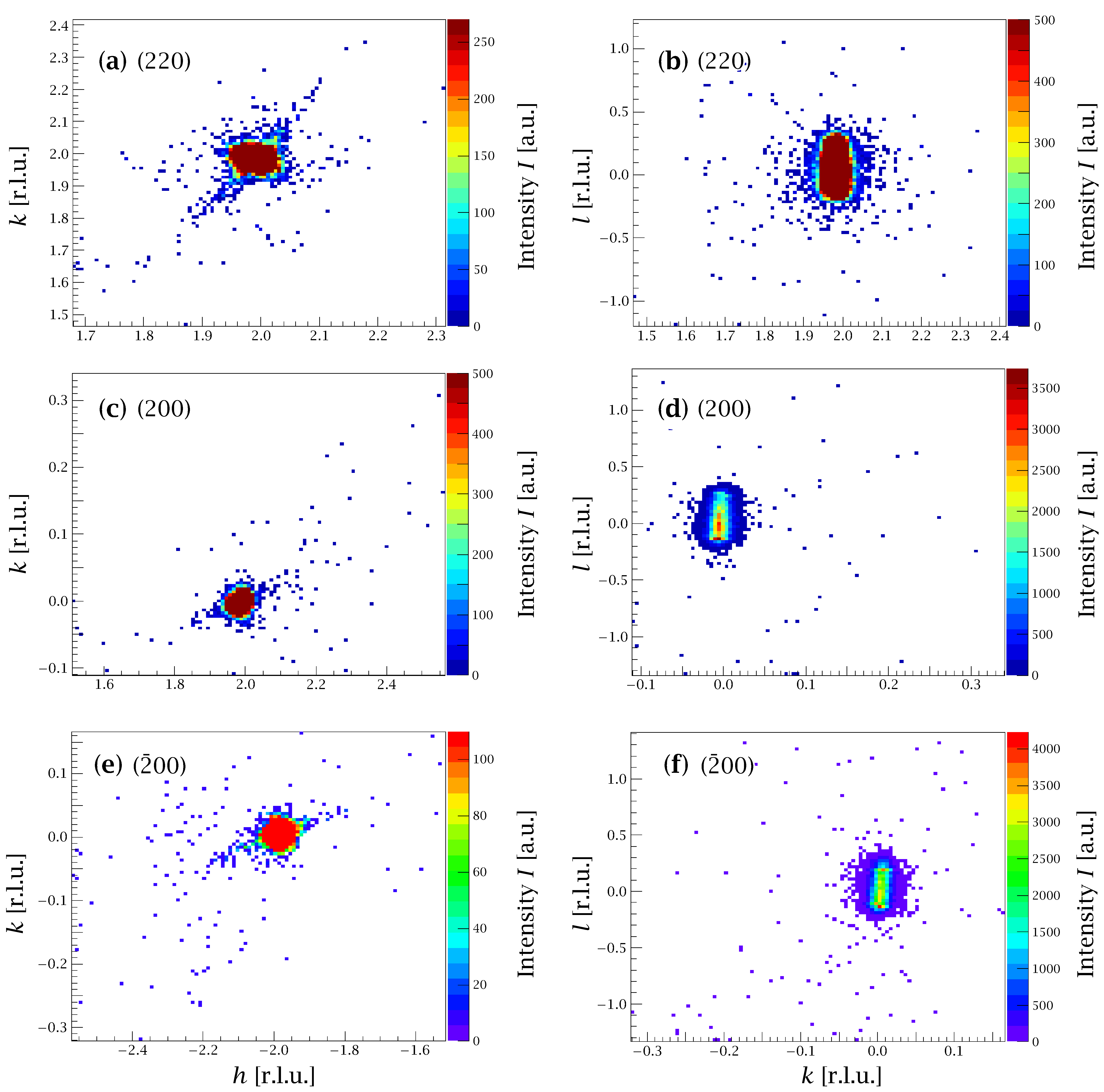
Figur 11.5: Scans of three peaks using the 2D detector at room temperature. Download links:PNG • SVG • PDF. .
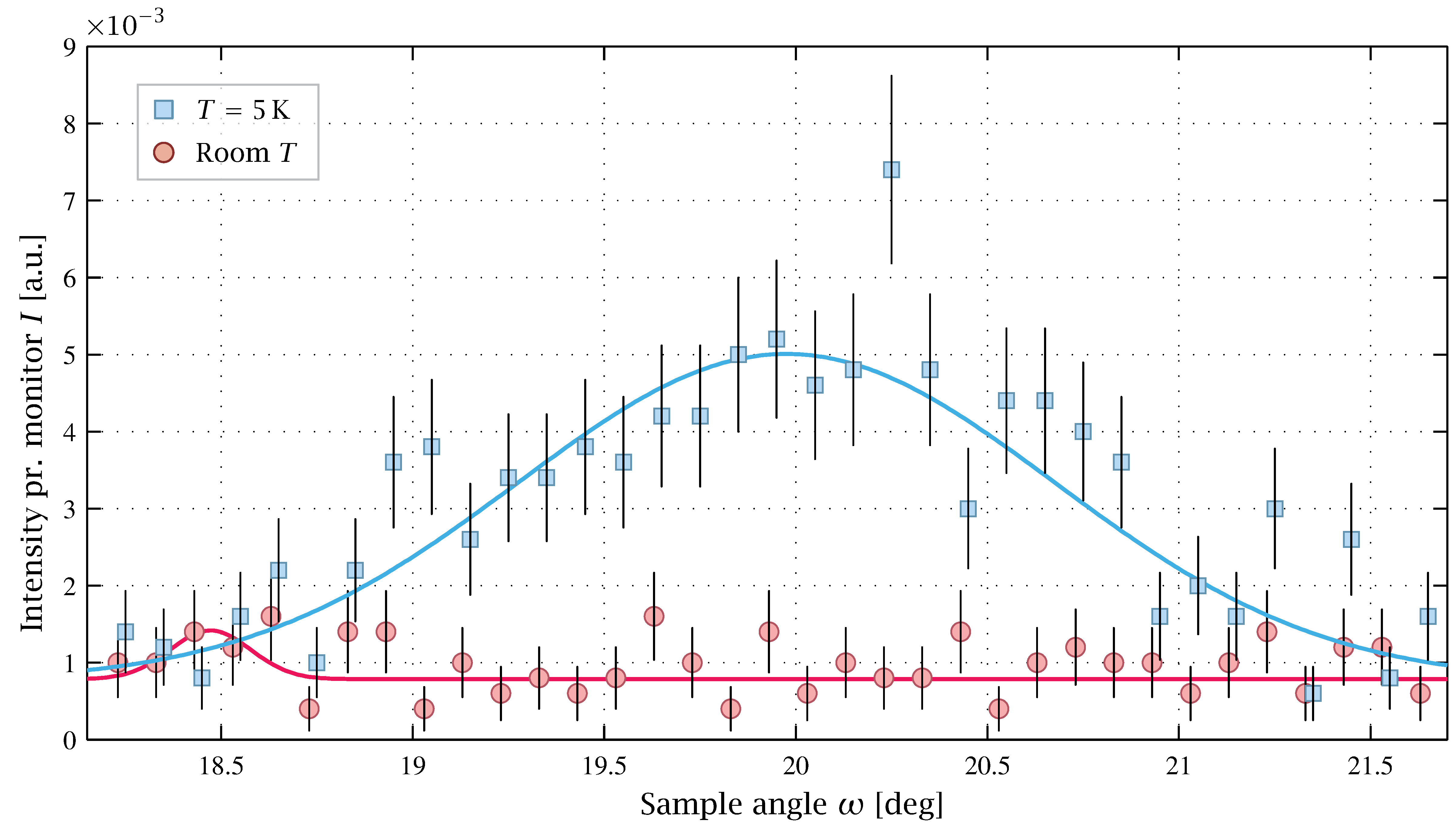
Figur 11.6: Measurement at Bmab peak location at 5 K and 300 K. Download links:PNG • SVG • PDF. .
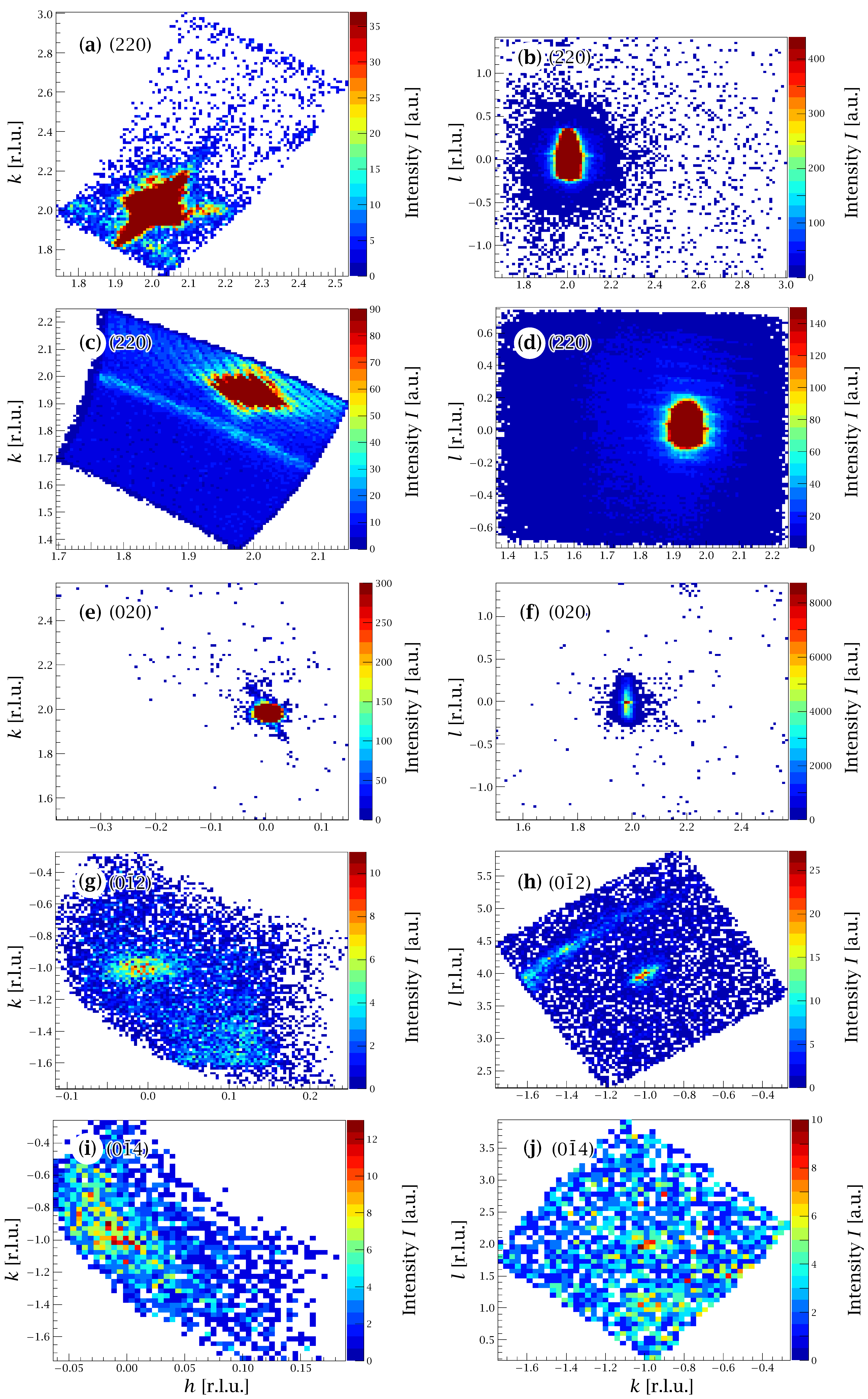
Figur 11.7: Scans of four peaks using the 2D detector at low temperature. Download links:PNG • SVG • PDF. .
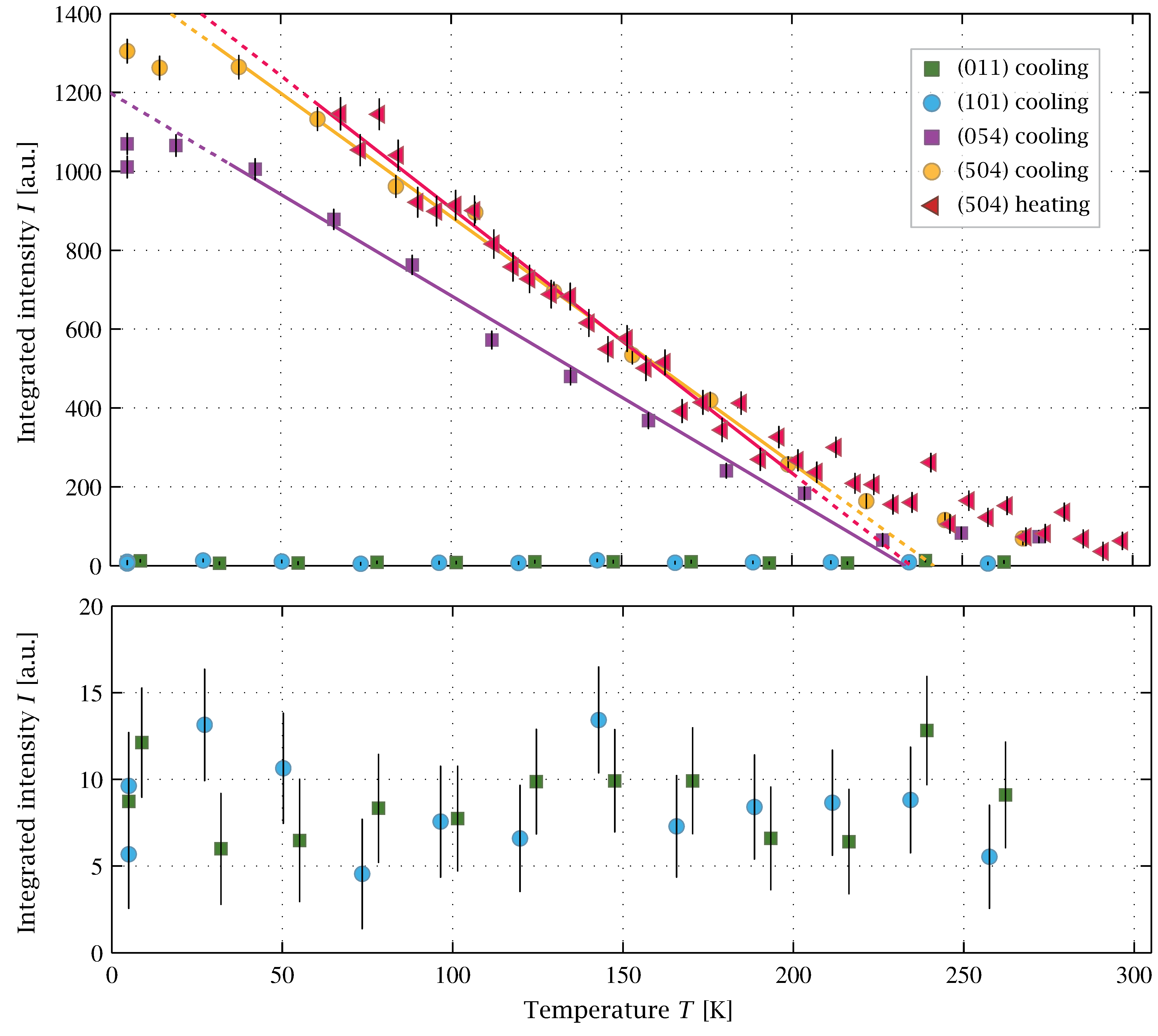
Figur 11.8: Measurements of (011), (101), (054), and (504) peaks as a function of temperature. Download links:PNG • SVG • PDF. .
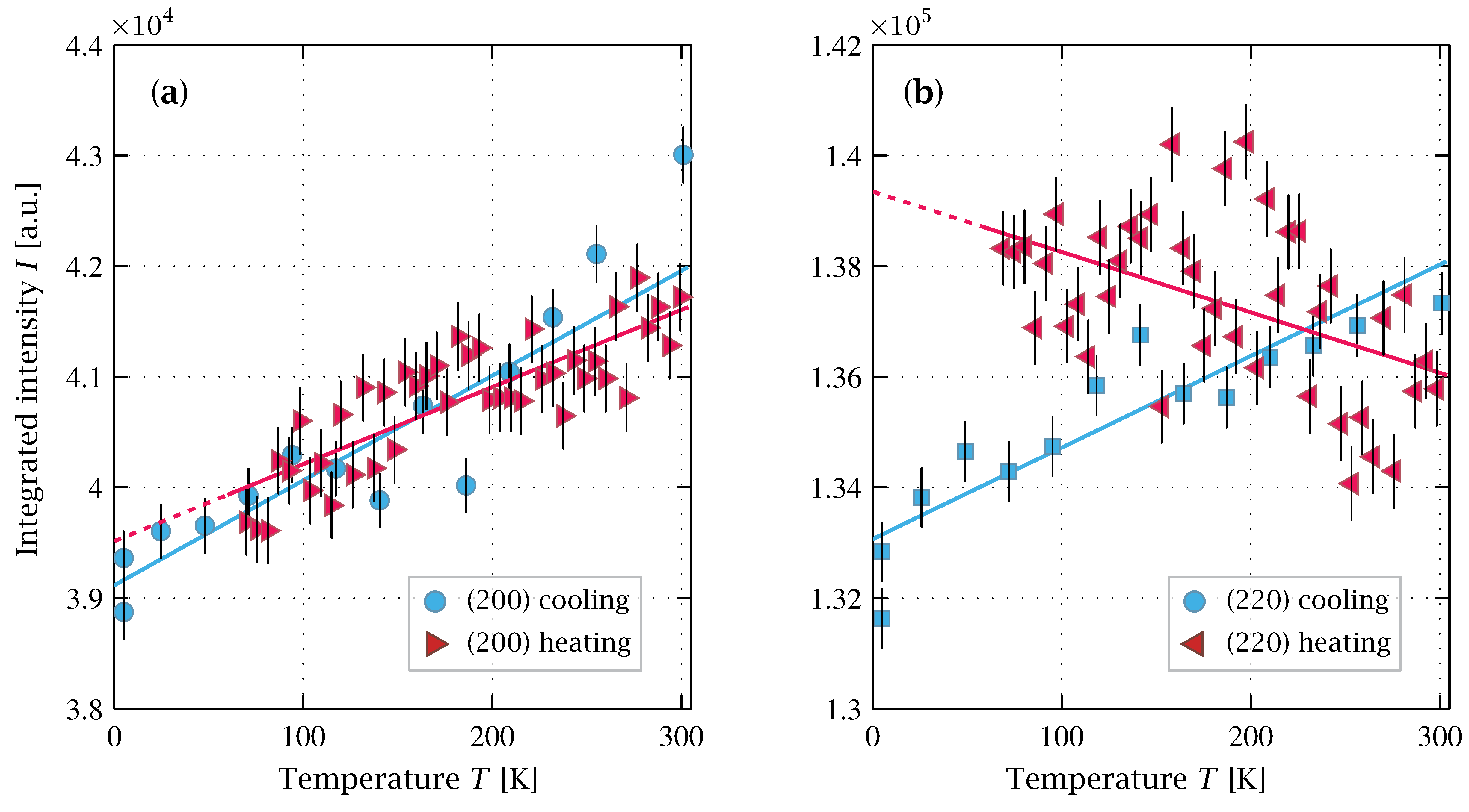
Figur 11.9: Measurements of (200) and (220) peaks as a function of temperature. Download links:PNG • SVG • PDF. .
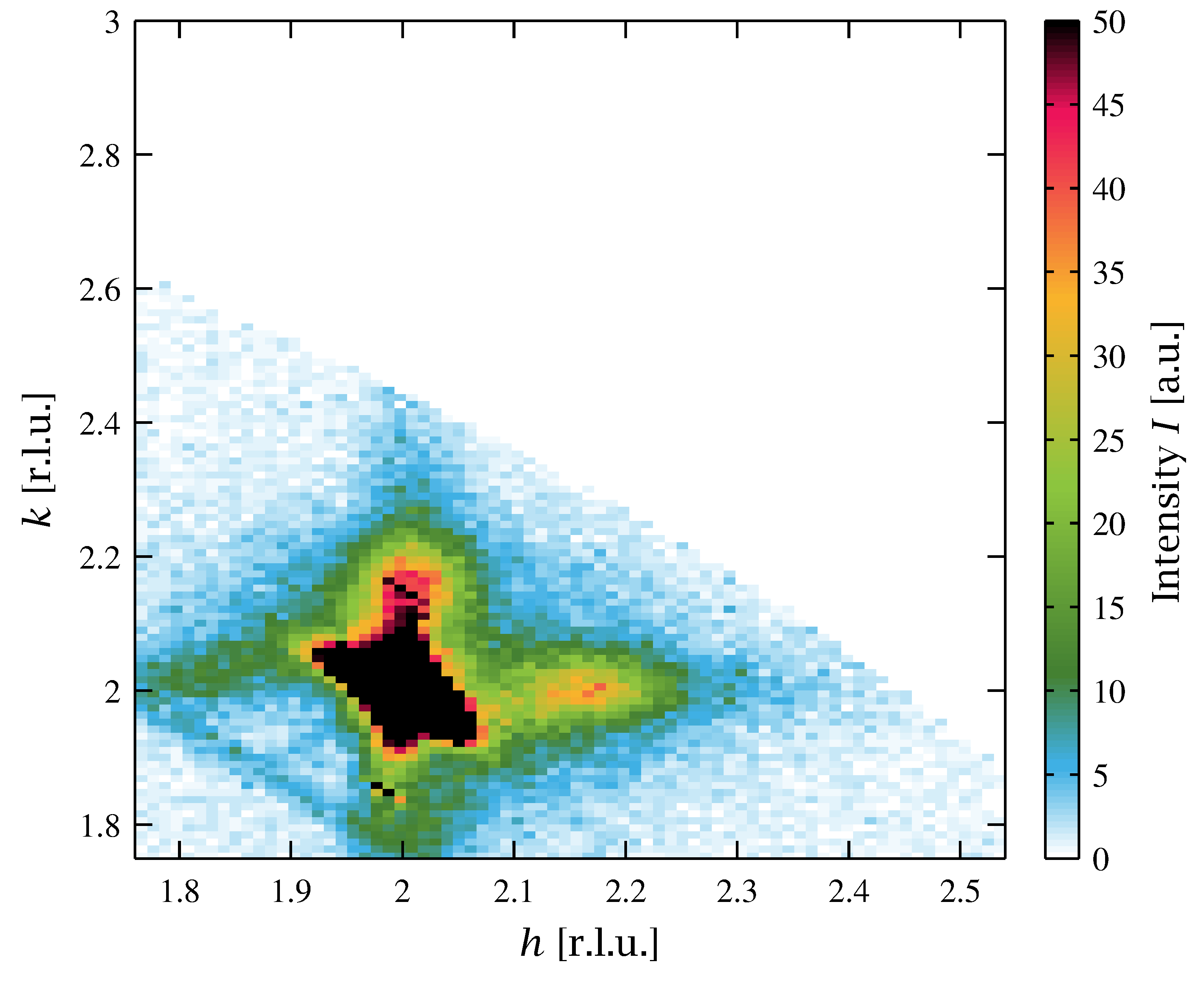
Figur 11.10: Zoom-in of (220) peak measured on DMC for La(1.94)Sr(0.06)CuO(4+y) at T = 2 K. Download links:PNG • SVG • PDF. .
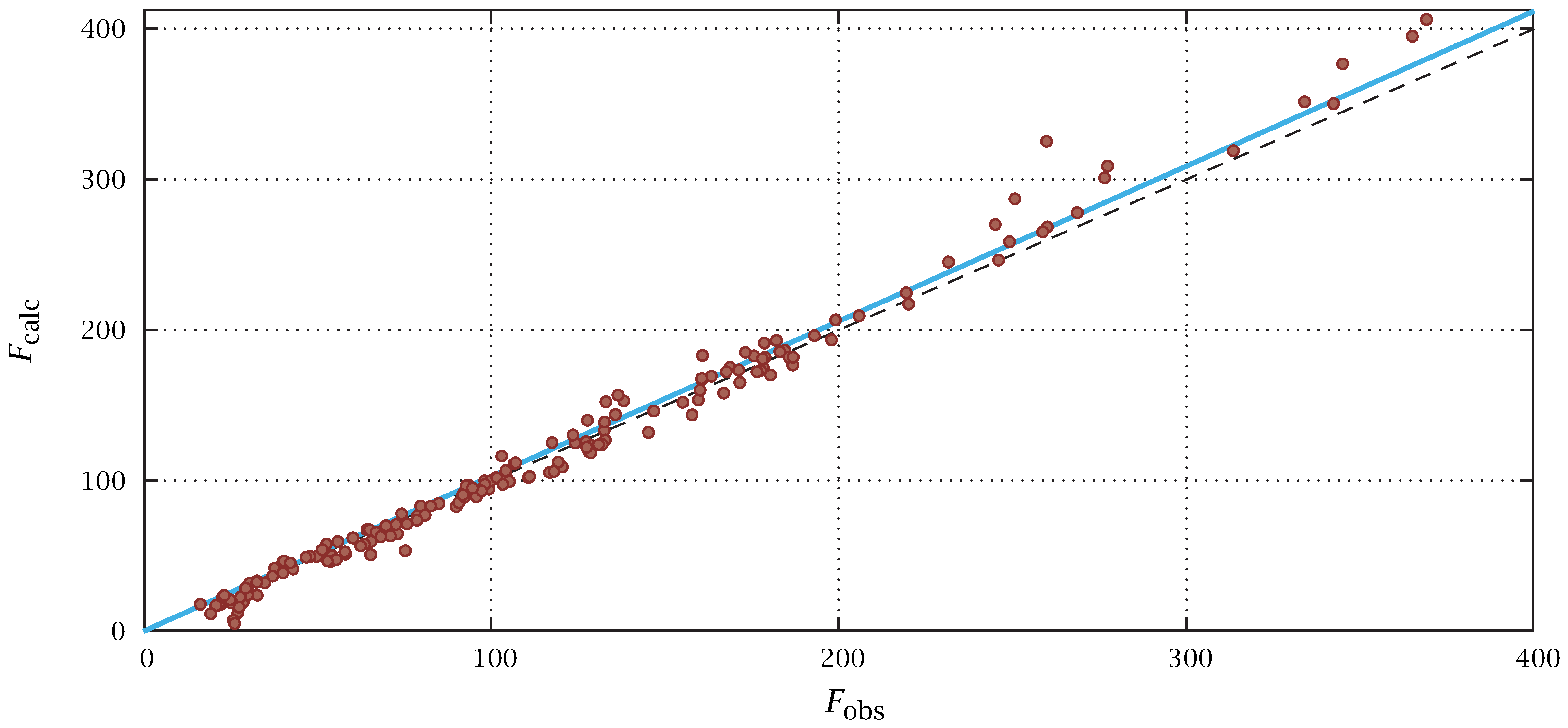
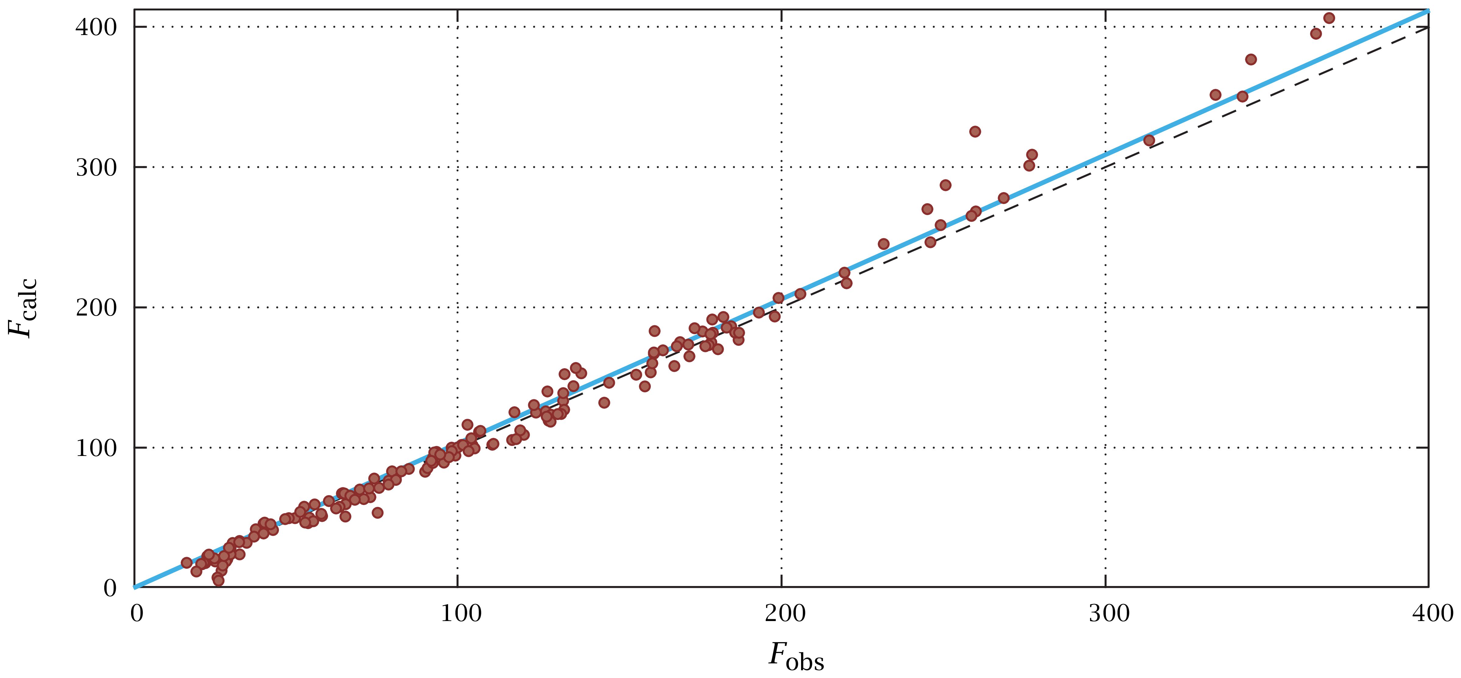
Figur 11.11: Fobs versus Fcalc values for the 300 K data set refined in JANA2006. Download links:PNG • αPNG • SVG • PDF. .
Diskussions-illustrationer (kapitel 12)
Figur 12.1: Comparing a standard unwarp with a background subtracted unwarp. Download links:PNG • αPNG • SVG • PDF. .
Figur 12.2: Comparing different integration thicknesses for lab. X-ray data. Download links:PNG • αPNG • SVG • PDF. .
Figur 12.3: Comparison of (0kl) and (h0l) planes. Download links:PNG • αPNG • SVG • PDF. .
Figur 13.1: Example of ID11 data frames. Download links:PNG • αPNG • SVG • PDF. .
Detaljer om prøver (appendiks B)
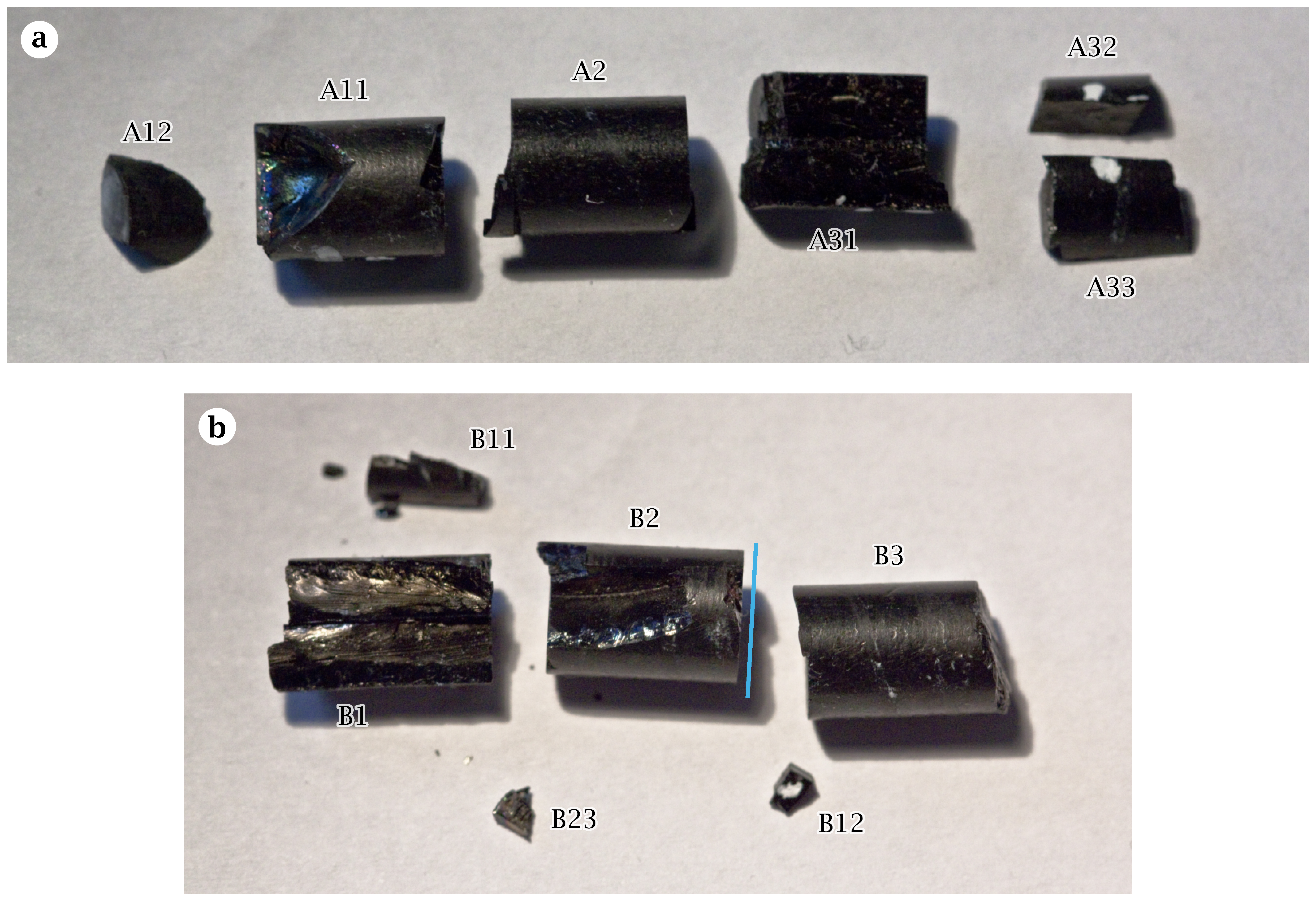
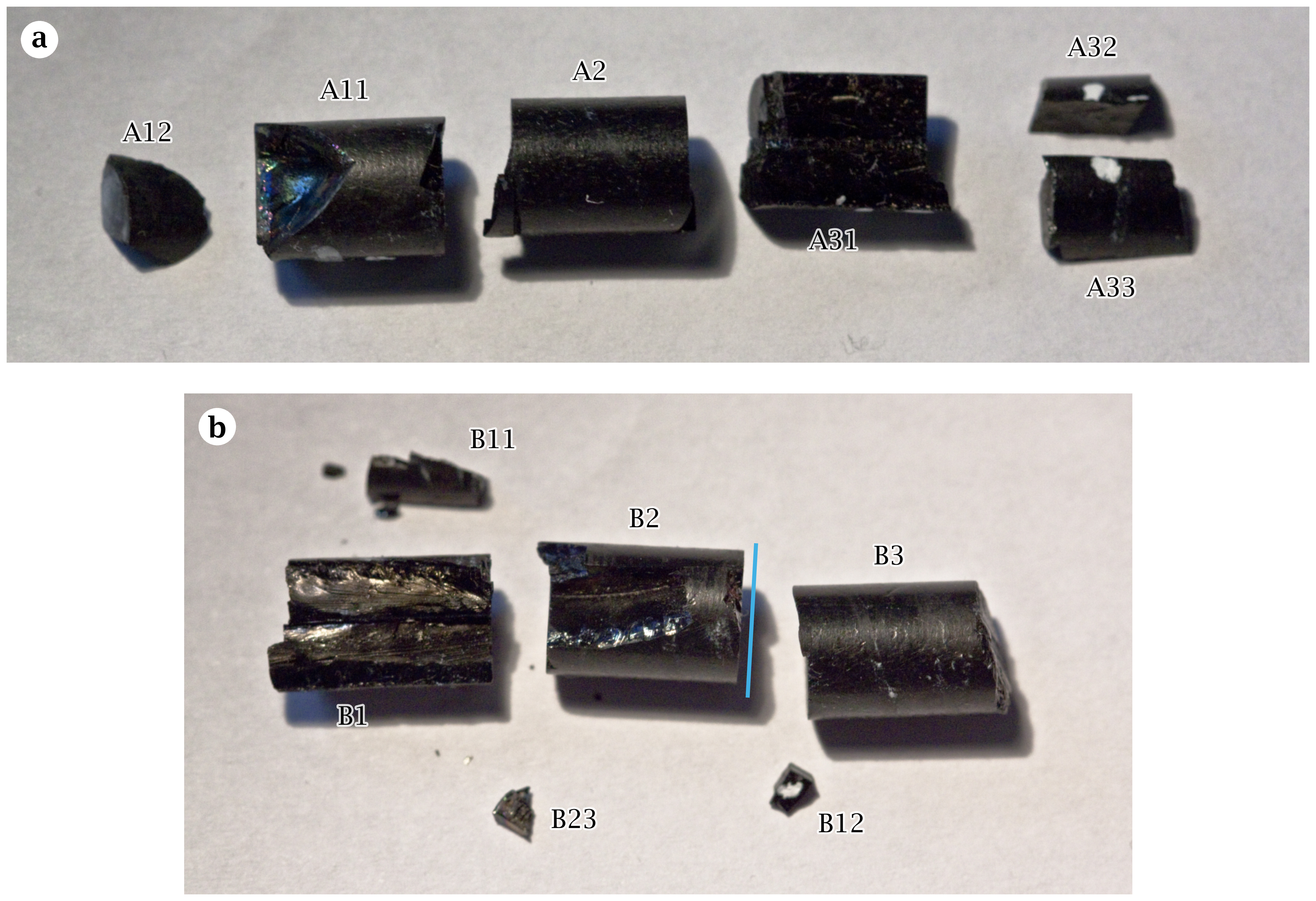
Figur B.1: Overview of the sLCO_DTU_A and sLCO_DTU_B crystals after cutting. Download links:PNG • αPNG • SVG • PDF. .


