Section 8 Exercise: Fourier and Wavelet Transforms

---

The exercise has four main purposes:

1. To show how Fourier Transforms work, and how they may be used to solve, for example, wave propagation problems.

2. To demonstrate the concepts of power spectra and auto-correlation functions.

3. To show how Wavelet Transforms work, and how they can be used to obtain information about wave modes in non periodic data sets and for compressing information with a "minimum" of loss and maximum compression.

4. To demonstrate how to use IDL X-widgets to build a graphical user interface to an IDL experiment.

Here are your 7 bonus points   Credits: 7/7

To extract the exercise files for this weeks exercise, do

    cd ~/ComputerPhysics
    cvs update -d

In case of problems, see the CVS update help page.

• The basic principle behind using FT transforms is that the base functions (Cos and Sin) represent an orthogonal bases. As shown in NR this requires the integral over the domain of the product of two different eigenfunction to produce a zero value for the integral.
• Start IDL/IDLDE in your ComputerPhysics/8_Fourier directory and run the products.pro program to explore if this constraint is fulfilled. The procedure shows why you need to integrate over the full length of the domain to reach the correct result....

  Is the mean of the product always 0 or 1/2? yes no Credits: 1/-1 OK

• You need a minimum number of points to represent a wave with a given wavenumber. Running aliasing.pro you can experience how waves with a higher wave numbers than the so-called Nyquist value are totally equivalent with lower wave number waves; they go through the same points.

  So, if you have a case with 8 intervals (as in aliasing.pro) and you choose a wave with 6 wavelengths ...

  .. this goes through the same points as a wave with 1 wavelength 2 wavelengths 3 wavelengths Credits: 2/-2 OK

• Run the play.pro example in IDL.

• Try varying, one by one, various Fourier coefficients from zero to non-zero and back again. Try both small and large wavenumbers. Note in particular how the high wavenumbers (close to the last, i.e. the Nyquist wavenumber) correspond to waves that are very badly resolved in physical space, but that these waves are represented EXACTLY in Fourier space.

• Try setting first one, then several Fourier coefficients nonzero and press PLAY (set by "dragging" points in the transform window). Look at the time behavior of the coefficients and the function.
  • Use the sliders to control the animation speed.

• Draw arbitrary functions (by "dragging" the function values), and watch the time evolution.
  • Note that the wave form returns EXACTLY to the original one after one period of evolution. This illustrates that all wavenumbers (including the ones corresponding to the "badly resolved" waves) are evolved exactly in the Fourier domain.

• Edit the play.pro file, and introduce damping, as discussed during the Lecture:
  • The place to look for is where there is a factor cos(omega*t); this is where you could insert an additional factor *exp(-eta*omega*t), where eta is a damping rate.
    • How large should eta be? Well, omega*t = 2*!PI, corresponds to one period, right? So, if you take eta = 0.1 or something like that as an example, the damping is a factor exp(-0.2*!PI) = 0.53 per period (not per unit time).
    • Try this out by adding a line "eta = 0.1" first.
  • Next, let a slider control the damping parameter eta and play with the parameters. Do this either ...
    • ... by "stealing" one of the existing sliders ...
      • Pick one of the sliders that already exists, and just change the name of the variable that the slider controls (only at the place where it picks up slider values), and then use the new variable (e.g. damping) in an expression such as exp(-0.001*damping*t*omega), to make the damping proportional to the period for each component (the factor 0.001 is there to make the damping small enough --- you may want to change it, depending on the range of the slider).

    • .. or by making a new one. You can copy from the existing code:
      • Duplicate the line that creates a slider, and change the names for it.
      • Duplicate the section that picks up the slider value, and change the name of the variable that the slider controls accordingly.
      • Then use the new variable in an expression such as exp(-0.001*damping*t*omega), to make the damping proportional to the phase for each component (the factor 0.001 is there to make the damping small enough --- you may want to change it).
      • NOTE: If you extend an IDL common block with a new variable, it is necessary to either restart or reset IDL -- common blocks cannot be extended while they are in use. To reset IDL, give the command .reset (note the dot).

• Set the slider so that the ground tone is damped by 50% when the animation stops (use trial-and-error, or compute what your slider should be set to).

  
  Try answering the following question. It is hard to see directly in the plot, but you don't have to; you can deduce the answer from what "overtones" means, counting on your fingers (careful now, this is a tricky question):

  With what factor has the 4th overtone been damped ? 1./8. 1./16. 1./32. Credits: 2/-2 OK

• Examine the signal.sav data, by following these instructions.
  • NOTE: It IS possible to cut/paste from the browser window. However, for each command, think about what it does rather than just executing it blindly.

  IDL> !x.style=1                              ; exact y-axis
  IDL> !y.style=1                              ; exact y-axis
  IDL> !p.multi=[0,3,2]                        ; 3 by 2 frames in a window
  IDL> window,xsize=1024,ysize=650             ; big window
  IDL> restore,'signal.sav'                    ; restore saved data
  IDL> contour,signal                          ; signal is a fltarr(1024,32)
  IDL> f=signal(*,10)                          ; one line of data
  IDL> plot,f                                  ; plot it
  IDL> plot,abs(fft(f,-1))^2                   ; plot its power spectrum
  IDL> plot,abs(fft(f,-1))^2,xrange=[0,200]    ; lowest 200 frequencies
  IDL> plot,fft(abs(fft(f,-1))^2,1),xr=[0,150] ; autocorrelation over 150 days
  

  • If these data represent 1024 days, then ..

    .. what is the Nyquist frequency (apart from the 2π factor)? 1/1024 1/512 1/2 1 Credits: 2/-2 OK

    Here's a hint about the Nyquist frequency   Credits: -1/-1

• Compute the power spectrum and the autocorrelation function for each latitude:

  IDL> power=complexarr(1024,32)
  IDL> auto=complexarr(1024,32)
  IDL> for i=0,31 do power[*,i]=abs(fft(signal[*,i],-1))^2
  IDL> for i=0,31 do auto[*,i]=fft(power[*,i],1)
  

  A pattern is obvious in surface and contour plots of power spectra and the autocorrelation function.

  IDL> surface, power[0:100,*], xtitle='frequency', ax=70, az=10
  IDL> surface, auto[0:100,*], xtitle='time', ax=70, az=10
  IDL> contour, auto[0:100,*], xtitle='time'   ; not so neat, but easier to read from
  IDL> contour, auto[20:40,*], xtitle='time'   ; zoom in
  IDL> plot,fft(abs(fft(f,-1))^2,1),xr=[0,150] ; autocorrelation over 150 days
  

• The data resembles what would be obtained if one measured the darkness of sunspots as a function of time (in days) at the central solar meridian, for latitudes ranging from the equator towards the pole. Judging from these particular data (estimating from the plots --- it may be better to use contour plots than surface plots for this step) ...

  .. what is the rotation period (within 5%) at the equator (lowest latitude)? Credits: 2/-2 OK

  .. what is the rotation period (within 5%) at latitude 30 (highest latitude)? Credits: 2/-2 OK

• To start examine the usage of wavelets, we are going to use the IDL provided tool for doing various wavelet analysis on different data types.

• Start the wv_applet in IDL. This opens a new window with a top menu bar, a bar with graphical icons and an area where information about the loaded data sets is available. Right from the start two datasets are loaded into the tool (called Chirp and Convection). You click on the name bar to active the one you want to work with.
• The icon bar is divided into smaller groups. Move the cursor over the icons to get a short text string indicating which action the icon represents.
  

• Click on the View Wavelet Functions icon in the 4th icon group. This opens a new window, where you can see the form of the different wavelet families and their dependence on their "order".
  • Look at the different wavelet families and how their general characteristics change as the slider is passed from left to right. Notice also the information given in the text frame.

• Start by examining the Chrip data set. This represents a 1D sinosoidal wave with a decreasing wavelength as a function of the data points.
  • First click on the 3D Wavelet Power Spectrum icon (the "box-like" icon in the 4th group). This opens a new window. To the left there is a graphical representation of the result and to the right there are possibilities for changing wavelet options and appearance of the image -- notice that the image is a real 3D image that can be rotated, translated or enhanced in size by using the three mouse bottoms.

  • The image consist of several parts. At the back is a 1D representation of the data -- the sine wave. In front the colour scale indicates the amplitude of the wavelet coefficients in the central surface plot. The x-axis on the plot (Time) gives the times at which the measurements of the sine curve were obtained. The y-axis (Scale) represents the time interval over which the wavelet has found the signal to vary.

    Choose the Morlet wavelet with the smallest order. This shows that the power peaks at time 180 with a signal length of order 64 and with a long tail extending into shorter scales for increasing time. This indicates the decrease in wavelength of the sinusoidal wave with increasing time.

  • Play with both the choice of family and its associated order and notice the large differences in the power spectrum between the different choices. The power spectrum using the correct choice of wavelet is good at showing how the sine waves frequency changes with time.

    Which of these wavelets would you choose for timeseries analysis? (more than one good choice) Deubechies Haar Coiflet Symlet Paul Morlet Gaussian Credits: 2/-2 OK

  • The next tool to investigate is the denoise tool that you access from the Tools menu in the top bar of the main window. A new window appears with many sub areas included. The top left image is the original data. The top right is the reconstruction of the image after removing noise -- high wave number information -- from the wavelet transform before calculating the inverse wavelet transform. The lower left image shows the amplitude of the different coefficients in the wavelet decomposition, while the lower right shows the histogram distribution of amplitudes as power and cumulative power in percent. The right hand side panels, again, allow choosing between a limited selection of wavelets. Use the percentage slider or coefficient number to limit the information available for reconstructing the time series.

    By just changing between the different wavelets (it chooses a specific order by default) and choosing 80 coefficients, which of these wavelets gives the best representation of the original data? Deubechies Haar Coiflet Symlet Credits: 2/-2 OK

• Click on the 2. Convection to select the 2D data set for analysis. This data set represents a shell model for convection in the mantle of the Earth.
  • This time we start the analysis with the Denoise tool. The reason is that this provides us with an image of the convection pattern. Notice the structure of the coefficients. In the upper right part of this image there is a clear selection of amplitudes inside a nice ring. Moving away from this corner the ring is repeated but with different sizes and aspect rations. This represents the sampling of wavelets amplitudes as the wavelet smoothing is increased over larger and larger fractions of the domain as indicated in figure 13.10.7 in NR.

    Choose the symlet wavelet and 750 coefficients. Which order of the wavelet gives the smallest percentage difference between the original and filtered image? 1 2 3 4 5 6 7 8 9 10 11 12 13 14 15 16 17 18 19 20 Credits: 2/-2 OK

  • Use the Import under the File menu to pickup some of the other data sets IDL provides for online testing. Notice that different data formats can be read into the wn_applet for further data analysis. Notice for instance how large a difference there is in the selected wavelet amplitudes between the convection image and the house image.

where f is the function and T is the time interval over which the function is to be analysed. Integrating this with different values of tau, large values are only obtained when tau represents time differences equivalent to repetitions in the signal of f. From this we define the wavelet autocorrelation function:

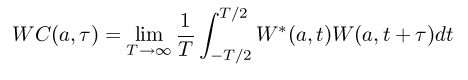
where W in general is the complex wavelet transform of a function. Here we are only interested in the real part of the wavelet autocorrelation function. In the wavelet transform a represents the different "time" scales over which the wavelet kernel is applied (see fig 13.10.7 in NR). Numerically data are represented by discrete values along the "time"-axis, and here the integrals transform into a sum.

To test it out lets start looking at a single sine function:

IDL> x=findgen(1024)/1024.                        ; define x [0,1[
IDL> fx=sin(x*!pi*2.)                             ; single sinewave
IDL> plot,x,fx                                    ; plot sinewave
IDL> w = wtn(fx,4)                                ; make wavelet, Deubechies, 4th order
IDL> cw = w                                       ; array for containing AC function
IDL> for i=1,9 do begin for j=0,2^i-1 do $        ; calculate AC function
IDL>      cw(2^(i-1)+j) = total(w(2^(i-1):2^i-1)*shift(w(2^(i-1):2^i-1),j))
IDL> cwcw=fltarr(512,10)                          ; array for expanding the information
IDL>                                              ; spread for easy plotting
IDL> for i=1,9 do cwcw(*,i) = rebin(cw(2^(i-1):2^i-1),512) 
IDL> tvscl,rebin(cwcw,512,100)                    ; rebin in y direction for more pixels

Can you use other values for the size of the second index of the cwcw then 10? (for this specific data set!) Larger Smaller No Credits: 1/-1 OK

Try a few more combinations to get more familiar with the information in the AC plot:

• Extend the definition for fx to contain more than one wavelenghts.
• Add a modulation of the amplitude of the sine wave with a different wavelength than the main modulation. The amplitude needs to be of a minimum amplitude to be easily visible in the tv plot --- if you rescale each wavelenght band this is not required.

  For this you want a different color table to make it easier to see small amplitude variations. Try the various ones to find one that fits the purpose, you can do this using xloadct.

IDL> w = wtn(signal(*,0),4)                                               ; Wavelet transform
IDL> cw = w                                                               ; array for containing AC function
IDL> for i=1,? do begin for j=0,2^i-1 do $                                ; calculating the  AC function
IDL>     cw(2^(i-1)+j) = total(w(2^(i-1):2^i-1)*shift(w(2^(i-1):2^i-1),j))
IDL> cwcw = ???                                                           ; array to contain the variable for plotting
IDL> for i=1,? do begin cwcw(*,i) = rebin(cw(2^(i-1):2^i-1),512)          ; stretching the information
IDL> tvscl,rebin(cwcw,512,100)                                            ; showing the AC in a position-wavelength plot

• Try to redo it with different orders for the wavelet.
• Do it for different latitude.

What do these AC plots tell us about the sunspots? Nothing Life time of sunspots That the data are difficult to understand using wavelets That the sun varies with latitude Credits: 1/-1 OK

• Earlier when playing with the wavelet experimentarium you made filtering of the chirp data. Now you are going to repeat the same analysis but using the FFT method.
  • Read in the data from the data file, chirp.dat.

    IDL> na=512                  ; Number of data points
    IDL> a=bytarr(na)            ; Define an array to contain the data (saved in byte format)
    IDL> openr,10,'chirp.dat'    ; Open the file for reading
    IDL> readu,10,a              ; Read the data (binary format)
    IDL> close,10                ; close data file
    

  • Use the same method as specified earlier to first define the power spectrum for the data.
  • Plot three different quantities in a single window showing:
    1. The raw data.
    2. The power spectrum, shifted such that the k=0 wave number is centred in the domain.
    3. The autocorrelation spectrum, with the same shift as above.

    IDL> window,0                                 ; opens window number 0
    IDL> !p.charsize=2                            ; doubles the character size
    IDL> !p.multi=[0,3,1]                         ; allows for three plot frames in the horizontal direction
    IDL> plot,a,xtitle='time',title='Function values',ytitle='Amplitude'
    IDL> ....                                     ; calculate the Power spectrum for a
    IDL> ...                                      ; calculate the autocorrelation function
    IDL> x=indgen(na)-na/2+1   ; define the x-axis for the shifted plots
    IDL> plot_io,x,shift( ??, na/2-1),xtitle='Wave number',title='....   ; plot the power spectrum
    IDL> plot,x,????
    

  • Each time you use a plot command, a counter is increased and next plot will be placed next to the previous one. The fourth plot will restart the circle and erase all previous plots on the screen. The first number in !p.multi=[0,3,1] (0) can be used to specify which frame you want to plot.... allowing you to replot at the same position in the plot window if you plot is not the desired one....
  • It is now possible to use the power spectrum as a guide to choose a level below which the amplitude coefficients are set to zero -- removing high frequency "noise" in the data. In this case this will instead remove information, such that the inverse FFT will not provide the correct result.
  • To be able to do this we need to do the following steps:
    1. Save the FFT of the original data.
    2. Define the threshold level for the power for which we want to set the Fourier amplitudes to zero and locate these wavenumbers and reset their amplitudes.
    3. Calculate the function from the altered Fourier coefficients.
    4. Plot the results of the different processes, and print the rms value of the difference between the original data and the truncated reconstruction of the data.

    IDL> window,2                                      ; opens a new window
    IDL> ff=fft(a,-1)                                  ; define the FFT of a
    IDL> level=.0100                                   ; define the threshold limit
    IDL> in=where(fa lt level, num)                    ; determine the k values in index space that needs to be zeroed
    IDL> plot_io,x,????                                ; plot the power spectrum
    IDL> oplot,??                                      ; a horizontal line indicating the cutoff limit
    IDL> if num gt 0 then ff(in)=0.                    ; set the chosen amplitudes to zero
    IDL> print,???                                     ; the number of non-zero amplitudes
    IDL> b=??                                          ; The inverse FFT of the truncated amplitude information
    IDL> plot,b,xtitle='time',title='Function values'  ; plot the truncated data set
    IDL> oplot,??,col=200                              ; add the original data set to the plot
    IDL> plot,???,xtitle='time',title='Differences'    ; plot the different between the two data sets
    IDL> print,rms(????)                               ; prints the rms value (real number) of the difference between the two data sets
    
    

  • By repeating a number of lines one can see how the reconstructed information depends on the truncation level.
  • This can be compared directly with the analysis done in the wn_applet using the denoise tool with the Symlet wavelet of order 4.
  • Remember the symmetry in wavenumbers in the FT of a real function before answering the following question!

    Choosing only 20 wave numbers for the wavelet application, how many Fourier coefficients does it require to get close to the same rms error between the original data and the filtered data? 30 31 32 33 34 35 36 Credits: 1/-1 OK

  • Visually compare the two results of the reconstructed function --- Notice how different they are despite having close to the same rms value. Which representation would you prefere?
  • Repeat all the previous commands into a single journal file called chirp.jou, with the addition that it prints the Power level, number of coefficients (ignoring the symmetry in the ft) and the rms of the comparison on a single line, the last line in the file! --- Only real numbers.

    Here is my version of chirp.jou Locate and upload your chirp.jou file: Credits: 5/-5 OK

Spend one of the reading hours of this week reading the chapter about Fourier Transforms and wavelet Transforms in Numerical Recipes. If you have a possibility to play with IDL at home, or by spending some odd hours at the Institute, then use the opportunity to play with the X-widget interface; modifying the play.pro example, or using examples from the IDL manuals, or inventing examples of your own.