Programming for Physicists: Exercise 9

Exercise 8: Final Project
Self-Organized Criticality

Last date for finishing all exercises and by that pass the course is:

Friday 6-11-2009
5 pm.

Introduction:

This is the last assignment of the course and provides your final chance for showing us that you have learned enough to write smaller FORTRAN programs. To pass this exercise you need to write -- from scratch -- a program that evolves a 2D system in a self-organized critical state (SOC). SOC has since it development in the late 80ties been used to address different dynamical systems that all are characterized by their non predictability. As examples of such systems can be mentioned the size and time distribution of earthquakes, large energy release events in the solar atmosphere known as flares, the size distribution of avalanches of sand grains on a pile of sand and even the stock prices. Like the game of life, SOC experiments are defined through a set of simple roles that alternates between stressing the dynamical system and releasing the stressed energy in locations where a predefined critical threshold is exceeded.
Having done the programming and tested the code, you have to write a short report describing your code, how to compile it, how to run it, how to visualize the results and show some example of the results. All of this will become more clear when reading the text below.

There is one condition that has to be made clear right from the start: This is a test of your capabilities of writing a Fortran code.

Therefore, the work has to be done individually, and not in groups!

It is not a problem discussing various issues with us or your usual mates, but you have to write the code, and solve the problems yourself.

Getting the required files:

Download the tar file to your ~/Dat_F directory and unpack it:

$ cd ~/Dat_F
$ tar -zxvf fortran8.tgz
$ rm fortran8.tgz
$ chmod 700 Exercise_8

This creates a new directory "Exercise_8" that contains the provided files for this exercise and allows only you to work with the content in it.

Self-organized Criticality

A simple setup to visualize is to have a disk and then drop sand grains onto it close to the disk center. As time goes a pile will appear and eventually it will form a cone with a close to constant slope. As new grains are added some will tumble down the sides before eventually finding a place to rest. Others will be more adventures and initiate an avalanche of grains that will slide down the side of the cone and vanish over the edge of the disk. In the laboratory one can construct this using a setup a little more complicated then shown in this cartoon:

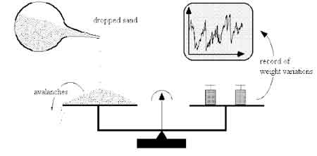
Using a digital scale one can monitor the changes in weight with time and associate the negative changes as measurements of the avalanche sizes. Making this type of measurements provides, in all SOC cases, a distribution function of the released "energy" that follows a power law with a given slope. Depending on the slope of the distribution function either the large or the small events contribute most to the "energy" loss from the system. Depending on the system, it measures different quantities and not all of them are in Joule. In the sandpile experiment it is the mass loss that follows a power law, while for flares, it is the released magnetic energy and for earthquake models the energy released in each event.

A problem with realistic models is that it is not easy to conduct experiments that work on realistic length scales and parameters. Instead model experiments are created trying to reproduce the behavior seen in reality. For earth quakes the simplest model is to take a brick, place it on a table and pull it across. This can be done by attaching a string with a force measuring unit to it. Then use a force that is just about balancing the friction, using a motor. If the force is just above the threshold for beating friction, the brick will move forward in "jumps" and the force measuring unit will change value dependent on how much forward the brick moves each time. The change in force is then a measure for the "energy" release and will result in a distribution function of force changes.
The expectation is that results obtained from this type of experiments can be extended to the large scale phenomena, implying the assumption that a SOC system does not contain a characteristic length scale.

A different approach to the laboratory experiments is to generate a computer model that analysis the same kind of system, allowing one to freely change the rules and control parameters to see how they influence the final result.

The best know SOC system is the sandpile. As it is also one of the simplest, we are going to make a model to simulate this on a computer. To do this we need a set of rules that can easily be applied and then ask the computer to repeat the basic event many time to improve the statistics of the distribution function.

In a scale invariant system one assumes the power distribution function to have no beginning (minimum event size) and no end (maximum event size). Neither of these assumptions are naturally true in reality. The lower limit is determined by the properties of the material involved in the process (atom size...) and the upper end relates to the maximum size of the unstable domain. Between these limits one expects the power law distribution to take up a significant fraction. That SOC systems have an inertial range (power law distribution) implies that the characteristics can be obtained from using relative small domain sizes -- in this case small numerical experiments and convergence of the result can be tested by simply doubling the numerical resolution of the experiment.

SOC sandpile model:
You are to reproduce a simple 2D sandpile experiment. To represent the disk, onto which the grains are dropped, you will use a 2D array of dimension (N,N). Where N is a variable number between different experiments. This array contains the number of grains piled in a column above this point on the plate. You should use one of two possible definitions of the disk.

Either assume a radius with a given size of N/2. This requires all 2D array elements with a distance larger than N/2 from the center of the array to be kept 0 as no grains are allowed to accumulate outside the disk.
Or instead use a square disk assuming that the outer perimeter is kept at zero value.

Adding grain at a single point, as is the default setup, creates a very systematic pattern. Instead we add a little noise onto this pattern by using Gaussian distributed random position centered on the disk (array) with a half width such that only a few grains (less than 1%) are dumped more than the give radius from the center of the disk. Grains are dumped one by one and the criteria for instabilities are investigated after each dump and eventual avalanches are allowed to evolve such that the pile of grains are always in a stable state before adding a new perturbation to the system. For each avalanche, the total mass loss across the chosen plate boundary is measured and its size is stored for later analysis together with the number of iterations it takes to end the avalanche event and the total number of cells involved in the avalanche.
This process assumes that the timescale for adding grains is much larger than for the avalanche to take place. This process, adding a grain followed by a relaxation of the pile, is repeated many time, such that a sufficiently large number of events are registered in the data base. The simple analysis of the data is simply to make histogram counts for the results and present them in a plot.

All the above is just describing the situation in words. To actually get this to work, you need to see the rules that initiates the avalanches and keeps them going until a new stable configuration has been reached.
Use the 2D variable z(x,y) to contain the number of grains at a given location. Use the random generator to chose a location to add one more grain

z(x,y) -> z(x,y)+1

z > z_crit

z(x,y)=z(x,y)-4
z(x+/-1,y)=z(x+/-1,y)+1
z(x,y+/-1)=z(x,y+/-1)+1

As you can see from the rules above, adding one grain to a given position in the grid changes only this points value and possible to a value above the instability criteria. Therefore after adding a grain one only has to check if the new z value exceeds the critical value. If this is the case, grains are to be redistributed accordingly and one must subsequently investigate the 4 neighboring points to see if any of them exceed the criteria. Each instability gives rise to a ring of points that needs to be checked as they can potentially have become unstable. This process continues until no new points are unstable. To prevent this process to continue infinitely, special care must be take at the edge of the chosen domain, where the grains placed outside the physical domain represents the grains loosed from the pile. Adding these gives the size of the avalanche, after which these must be reset to zero.

Lets bring this into a more concise formulation of the problem:

Give input values for:
- The grid size
- The % radius of the disk onto which the initial grain can be added
- The number of grains to be added in the experiment
Arrays and structures
- Allocate the array to handle the counter of grains
- Create a mechanism to handle the points that may become unstable when grains are redistributed due to a local instability
  - This may be done in two different ways -- an efficient way and more cpu expensive way
  - The efficient way:
    - Use a sorting tree like in the previous exercise
    - Define two structures which can be used to sort the possible unstable points
      - This can be done in two steps:
        
        One that sorts the incoming points according to the x position.
        A perpendicular set for each fixed x position that makes a sorted list in the y position
      - Keep track of how many points are added --- some may be repeated several times and only need to be counted once, that is what the list above is meant to do for you
      - Read the list of points back from the tree structure and use this as input for testing the gridpoints for instabilities.
  - The less efficient way:
    - Use a 2D array of type logical. Default value is .falsh.
    - Set the neighboring points to an unstable gridpoint to .true. and then impose this redistribution formula on these points
    - This requires to investigate all points in the grid
Iteration process
- Choose a position to dump a grain
  - Use a Gaussian random number generator to provide two random numbers (see below what is need to included it in the code)
  - Use the random numbers to move the actual dumping point within a given percentage of the mid point of the 2D z array
  - This is to avoid getting a to symmetric evolution of the system (The tradition is to use the central point all the time...)
- Update the grain counter at the chosen point
- Define the list of potential sits to be tested for instabilities
- Check the potential points for instabilities, if it/they is/are found to be unstable
  - Redistribute the grains according to the description above
  - Add the involved neighboring points into a new list to be checked for instabilities
- Keep track of how many grains have been pushed over the edge of the domain before the pile has again reached a stable state -- the avalanche size
- Keep track of how many individual cells are involved in the total redistribution
- Keep track of how many iterations it takes to relax the system
- Save the three numbers for each grain loosing avalanche in a file for later analysis --- three numbers per line in a file.
- Redo the dumping of a grain and the succeeding relaxation until the required number of grains have been dumped

Traditional the instability criteria is set to z_crit=4. Making it larger makes no difference to the distribution function as it only provides an offset in the number of not changed grains in the z array.

Programming Assignment:

Before you start coding the final task, take the time to understand the information above. It is vital that you have a clear picture in your mind, or rather on paper, with regard to what needs to be done. Which conditions needs to be included and in which order. How can the program be structured, i.e. how can the problem be divided into small sub tasks and how do they all fit into the global puzzle --- you may benefit from making a pseudo flow diagram of the code you have to write. When this is in place, there are a number of requirements to the way the program is written:

Program requirements:

Main program controlling the calculations
Subprograms for the actual calculations
- Use modules
- Bundle routines together in a way that make sense
  - IO, mathematics, sorting lists, ......
- Use namelists for input of the scalar input
- Use allocatable array(s) to allow for different 2D sizes of the "disk"
Allow the program the following flexibility
- Size of the 2D arrays used
- Max number of iterations allowed
- Size of the region in which the grains are dumped
Use a Makefile for the compiling of the program
Save the "relaxation time" of the event, the mass lose and the total number of cells involved in the relaxation later plotting with idl or gnuplot
- For idl use the plot.jou journal file. Before using the journal, you need to specify the name of the data file and the number of events to be read in. You have to change the labels of the generated figures. Finally, there is a typo in the last line where you have to remove the file=.

You have two options. Either write everything from scratch or get a little help. The most tricky part in the program is setting up the double sorting tree structure. It can be done as a careful extension of the sorting program you worked with in the previous exercise. The other possibility is to download this tar file to your exercise directory, which contains a not all working file that may help you on the way to a fully working list handler.

To use the included random number generator you have to do:

This returns one Gaussian distributed real number in the variable tmp with a mean value 0 and a 99% likelihood radius of 3. Scale the radius to a given percentage of the domain size and add an offset to place it at the center of the domain.

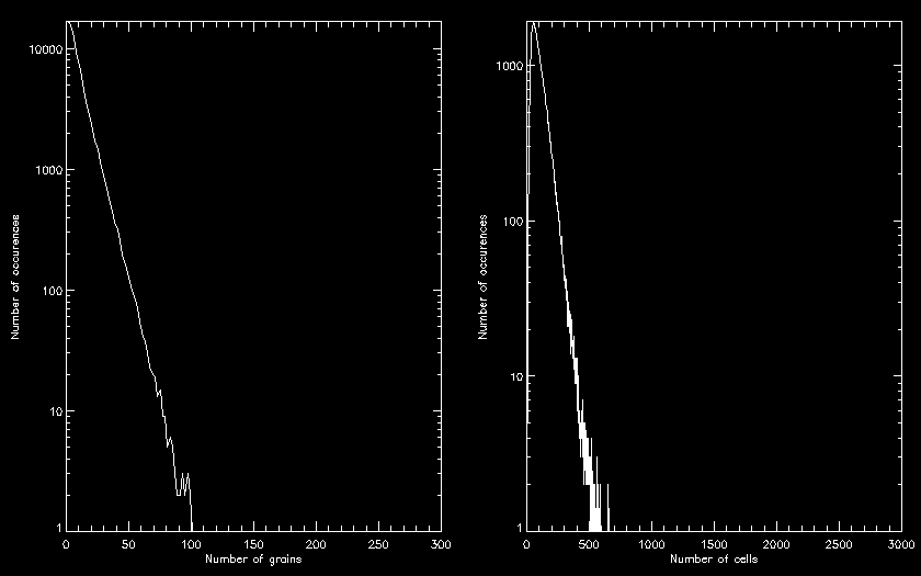
A simple test run that show the distribution functions can be done using a grid of size 50 and 1/2 a million grain dumps. Allow the dumping region to be on the order of 5% of half the grid dimension. Using the fast approach for tracking potentially unstable points, it should run in about a minute.

This is the results I get using plot.jou, with the values above:

Report:

Apart from the programming part in this exercise, you are also required to write of a short report. The report is supposed to provide the information outlined below, showing that you have an idea about the basic problem, the layout and use of the working program. Further to this there must be a description of how to compile and run the program and how to generate the included plots. This report has to be detailed enough that one of your fellow students not following the dat-f can compile and use your program to reproduce the plots. Here is a list of headlines to address in the report:

Introduction to the problem
- What is SOC
- What is the idea with this report
Description of the program
- How does it work
- How to compile it
- How to use it
- Known limitations
Proof that the program works
- Include plots showing the distribution functions of the avalanche sizes in the experiment.
Final summary of the project
- Your perspective of the project and the final outcome

You are free to write the report in Danish or English. With regard to the format of the report, it can either be provided as a pdf file, an openoffice or word document.

Before you are finished, collect all the files important for us to evaluate the project in a single tar file called project.tgz. For this you need to do something like this:

$ tar -zcvf project.tgz Makefile *.f90 Report *.in gnu_plot_scripts/idl_scripts

where the names after project.tgz represents the files you want to include into the tar file. You may want to include this in the Makefile and then only need to write something like:

> make project

I have packed the report and code into project.tgz and I am ready to submit it Credits: 1/-1

This time submitting the project file is not enough. Because your Exercise_8 directory is only accessible for you, the project.tgz file must be emailed to kg@nbi.ku.dk.

Finally, make a "cleanup" of the files in all the Exercise directories that are not required. Go into your Dat_F directory and use du -s * to find the large directories.....

References:

For the ones interested in the background material for the exercise:

Thank you for choosing Dat-F as one of your course in this block

The Dat-F team

$Id: index.php,v 1.7 2009/10/23 09:45:20 kg Exp $ kg@nbi.ku.dk