Exercise 6: Debugging and
Optimization
!! Electronic student evaluation of the courses !!
All
students are asked to login on the ABSALON web pages for all the courses
they follow in this block and fill out the evaluation form.
You
must do this within the period 9th to 26th October.
So why don't
you do it right now?! |
Introduction:
Making an error
free program first time round is not very likely -- as you all know by now --
and as the program package increases in size the likelihood for making mistakes
increases too. Errors can occur in many situations, some are easy to detect
while others are minor and only make a small signal on the final result.
Whatever characteristic the error has, you normally want to eliminate it to get
an error free program. There are different approaches to track errors. One can
take the simple approach by including print (or write) statements
into the program at relevant places. Recompile and rerun the program.
Investigate the output and determine where to put new print statements
while removing some of the previous ones. This way it is possible after a number
of cycles to get close to the area in the code that is responsible for the
problem. This approach works well, but it can take a long time. A different and
usually faster approach is to use a debugger. These come in two flavors.
The simple command language driven debugger, where you slowly step through the
program in a shell like environment, typing various commands. To use these you
have to learn all, or at least the basic, commands and generally to have one or
more editors open showing the source code as you work your way down through the
program statements. The second class of debuggers use a GUI, where it is
possible to see the source code, set strategic breakpoints and investigate
values of all local variables as you work your way through the program
statements. In this exercise we are going to try the last type of debugger
environment.
Getting the required
files:
Download the tar file to
your ~/Dat_F directory and unpack it:
> cd ~/Dat-F
> tar
-zxvf fortran6.tgz
> rm fortran6.tgz
This creates a new
directory "Experiment_6" that contains the files needed for the
exercise.
Debuggers:
A debugger is a
tool that can help you to see what happens in the code while it is running on
the computer. Before the debugger can be used on the code, it has to be compiled
in a way that the debugger can step through the code while providing useful
information about it:
- The actual location in the code.
- Shows the relevant source code.
- Provides access to variable values.
- Step through the code in various manners.
To reach this point,
compile the code with the option: -g. At the same time optimization of
the code has to be remove. Optimization gets the code to execute faster, but
this is often done by rearranging the order in which the statements in the code
are executed. This confuses the debugger and we can't be sure that the place
where the code seems to be in the debuggers graphical window is in fact also
where it is in the execution process. Therefore use only -O0 (capital o
and zero) when recompiling the code. When this is done we can use the debugger
on the executable to find problems in the code.
For today's exercise, you
have to debug and correct a number of typical errors placed in the program
included in the tar file. As you may already have see, the program is an
extension of the code you wrote for the three body problem in exercise 4. This
version includes the possibility for using both the simple expression for the
time derivative of the acceleration (eq(8)) and the full expression (eq(5))
given in that exercise and is able to handle more than 3 objects by using
allocatable arrays.
As a start, make the relevant changes to the
Makefile, such that the compilation has the correct options. Then compile the
code.
As you are already acquainted with the problem there is no
introduction to the problem here. If you do not remember the background, go back
and check it out in exercise 4.
To run the program from the prompt you
simply have to type,
$ ORBIT.x <
data.in
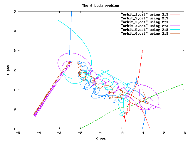
This is what the solution may looks like when you are
finished debugging the code and correcting the imposed errors. Only the left
half are likely to be identical to this one as only very small truncation errors
on different CPUs creates exponentially growing differences...
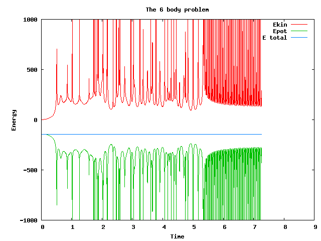
And this image is
just to show how the energy conservation is fulfilled for this
integration.
The section below
gives you information about how to use the debugger and find the problems in the
code.
Data Display Debugger --- DDD
The Data
Display Debugger (DDD) consist of a GUI interface that can use a number of
command line debuggers. DDD is a GNU product and it is as such made to use GNUs
debugger gdb. Initially gdb didn't support fortran codes as GNU product
didn't include a fortran compiler. But that has changed recently, so you should
in principle have two possibilities. Either to do the exercises using the
gfortran compiler, or use Intel's Fortran compiler, ifort. For
some reason the gfortran compiler doesn't allow you to do what is need in this
exercise. Therefore you must use ifort for this exercise. As a part of the ifort
package, there is also a more advanced debugger, idb. The older versions
of idb has both a command line and a graphical interface, while the
newest version, release 11, only provides an advanced graphical interface.
idb is gdb compatible, and that makes it possible to use versions
10 or less of idb as the underlying debugger for DDD.
Debugging
is a very important task in software development. The most important issue in
programming is to make a full proved program that can handle all possible
scenarios in a sensible way. Before this state is reached, it is normal that
there are parts of the program that for some reason do not behave as they
should, and therefore causes the program to either crash or provide you with
wrong answers.
To test a program you need to have a series of test cases
where you know the answer. Test the program against these and resolve eventually
problems that arises. When the numerical results are consistent with your
expectations, it is most likely that the program does what it is expected to do.
On the way to this you will, repeatedly, experience that various things do not
behave to your expectation. To find out where and why the error occurs you debug
the code.
We are going to use the ddd debugger interface this time. The
reason is that it is sufficiently simple to use that it does not requires a long
introduction, while still providing the basic facilities needed when debugging.
To start DDD using the Intel debugger, idb, you type
$ ddd
--debugger "idb -gdb"
using version 10 or older of ifort (which they
have at the fys.ku.dk at present. Or
$ ddd --debugger "idbc -gdb"
when using version 11 on lynx.
Using the gfortran and gdb directly
you only have to type
$ ddd
(For this exercise you
need to use the ifort compiler as there is a problem with debugging the
code I have provided using the gfortran compiler -- it does not all you to view
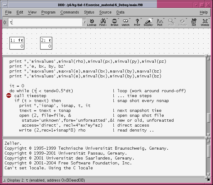
function values of dynamically allocated arrays.) This opens a window
containing three different sections (see the image below). The top one is for
displaying variable values, the middle frame hosts the source code, while the
bottom one contains the command line interface which includes the IO from the
running program. To load a program into the interface you choose File
from the top line. In the new window, click on open program and choose
ORBIT.x. This opens the source file of the main routine and puts the
pointer at the top of the main routine.
Before starting to
debug the code, you need to set a breakpoint in the source. This is a point
where the execution will stop and allow you to look at various values in the
code. You could for instance put one in the line containing the call
input. This allows you to see how the program reads the initial data into
the code. To start the execution choose Program from the top menu, and
then click on run. This opens a new window. In the lower input line you
must type
<data.in
which makes the code read the input
from this file.
At the same time a small window called DDD
appears (see the image below). The choices here are the ones needed for running
through the program.

|
| Command |
Impact |
| run |
Start running the code |
| interrupt |
Stop the execution now |
| step |
step one line at a time - going into underlying
subroutines/functions. It also steps into
standard fortran routines as print and allocate. To
avoid this use next to jump over these internal
routines. |
| next |
step one line, do not step in to routines
| |
| up |
Move one level up, if not at main level |
| down |
Move one level down, if possible |
| cont |
Continue execution |
| kill |
kill the process |
| undo |
undo the last command |
| redo |
redo the last command |
| edit |
opens the source code in an editor |
| make |
will in principle recompile the code,
but.... | |
To
see a value of a variable, place the courser on top of it and its value will
appear on the screen. To follow a series of values while progressing through the
program mark it with the cursor and click on display in the top bar. This
will place a copy in the top frame. The values shown here will be updated each
time the program stops. If you are dealing with a 1 or 2D array you may use
plot instead. This puts the variable in the top frame, while also
starting Gnuplot, which plots the data array in a new window - one for each
variable chosen. The plots are also updated each time the debugger stops.
To get the Gnuplot interface to work you have to change the default
settings. This is done by clicking on Edit and then choose
Preferences. In the window that appears you choose Helpers and
choose External for the plot window. You can remove the many
comments about x-applications by choosing Suppress X Warnings in the
General page in the Preferences window.
You are now ready to start finding the planted errors and
correct them.
To help you, here is a table showing the number of
errors placed in each files: |
| File |
# errors |
| data.in |
1 |
| main.f90 |
3 |
| data.f90 |
1 |
| timestp.f90 |
1 |
| io.f90 |
3 |
| math.f90 |
3 |
| orbit.f90 |
4 |
| Makefile |
2 | |
When
the program is running you can compare the results with the images above using
gnuplot in an independent window. Start with making shorter runs, only allowing
the solution to advance 1 or 2 time units.... If this seems OK you can do the
full 7 time units to get the same images -- before doing this
you need to change the options for the optimisations of the compiler from
-g to -O3 and recompile the code -- otherwise it will take a very
long time to run.....
Performance analysis
Now that the program is
working it is time to make a different investigation. Namely looking at the
performance of the code. There are different tools that can be used for this
purpose and here you will try one of these. As for the debugging, you have to
compile the code with special compiler flags to be able to sample the run and
obtain the data you need. For this purpose you have to change F90FLAGS to
F90FLAGS = -O3 -p
-O3 implies high optimization of the
code, giving a fast execution of the program -- you can try to use different
values after O to see the effect. Measure the run-time using the Unix command
time -- if you don't know how to check the man page.... The -p option
informs the code that it has to provide information needed for profiling while
running. For this to take effect the code has to be recompiled from scratch.
When you have done this, change the finish time in the *.in file to a smaller
time (=1) and run the experiment from the command line by typing
$
ORBIT.x < data.in > log
The result of this, apart from the
normal data output, is a file called gmon.out. This file contains
information for each short time interval (0.01 second) about where in the code
it was at that specific time. If this sampling time is short enough, and the
duration of the experiment long enough, it gives a fair picture of the time
usage in the various routines. To extract this information to an easy readable
format you have to do:
$ gprof -z ORBIT.x > gprof.out
This creates the file, gprof.out, which contains information
about the time usage in the various parts of the code, in ASCII format. Open
this file with a text editor and look at the numbers. Here is a small part of
the file, (for a different experiment!):
Flat profile:

Each sample counts as 0.01 seconds.
  %   cumulative   self              self     total
 time   seconds   seconds    calls  ms/call  ms/call  name
 57.53      0.42     0.42     7569     0.06     0.09  pde_
 15.07      0.53     0.11    98397     0.00     0.00  stagger_mp_xdn_
  5.48      0.57     0.04    52983     0.00     0.00  stagger_mp_ddxup_
  4.11      0.60     0.03    45414     0.00     0.00  stagger_mp_xdn1_
  2.74      0.62     0.02    98397     0.00     0.00  stagger_mp_ydn_
  2.74      0.64     0.02    45414     0.00     0.00  stagger_mp_zdn1_
  1.37      0.65     0.01    98397     0.00     0.00  stagger_mp_zdn_
  1.37      0.66     0.01    45414     0.00     0.00  stagger_mp_ddzup_
  .....
The first table in the file, from which the first few lines above are
shown, gives a sorted table of the routines according to their relative
percentage of the time usage during the run. The first column shows the
percentage of time used in the routine, the second the cumulative time and the
third the actual time spend in the routine. Some of the routines contain call to
other routines, and the splitting up of time in these are shown in tables
further down in the file. Using this information, it is possible to find the
routines that are using the largest fraction of time, and therefore are
potential targets for using your effort to see if it is possible to improve the
performance of the code. Depending on the problem, this may require rewriting
some of the routines, restructure others and possible looking for more optimal
re-usage of the variables when they are placed in the local ram.
The
program we are investigating is smaller than the one shown above, and the spread
in time consumption is not nearly as skew as for that case. But there are still
routines that uses more time than other routines and it is these and their
underlying routines you should concentrate on to see if you can find ways to
improve the performance. There is not one, but several smaller issues that
together can provide a nice speedup of the code. Lets make this a into a little
competition.... How fast can you get the program to run?
Some hints to
help you on the way:
- Check for loops where you do to much work
- Limit the number of floating point operations by moving constants outside
the do loops.
- Check for locations where you redo the same calculations more then once
- May require to define a new routine to compact the calculations
- Is it required to allocate and deallocate temporary variables each
timestep
For each of the files you are going to change to increase
speed copy them into a new file and alter the Makefile to use these (while still
being able to compile the old version when required)
To get the real
timing of the program on a multi user system, you can't rely on the timing gprof
provides -- it simply clock the usage of real time. This time includes idle time
on the CPU without being able to tell you how much time is spend waiting on
other processes. Therefore run the profiling a few times and look at changes.
The time command gives you information about how much CPU-time relative
usertime the program has used... It is the CPU-time that is important here.
The code you have used here uses dynamical memory allocation. Rewrite the
initial code (that you backed up earlier) to use static arrays -- predefined at
compile time -- and allow for only a fixed number of objects.
Before you are finished, try to change between the two compilers (ifort
<-> gfortran) and compare the execution time.... As you can see then it is
not only a task of optimising the code, but it also depends significantly on
which compiler one used for the actual run.
Cleanup!
Finally, just a reminder to clean up
your disk space by removing all the data files etc that are not needed any
more... You may also have some left overs from the last few exercises..... So
please, spend a few minutes to cleanup......
$Id: index.php,v 1.7 2009/10/09 08:03:01 kg Exp $ kg@astro.ku.dk