Exercise
5: Data IO
Introduction:
Data
input and output (IO) represents a very small fraction of most programs, but the
effect of IO is very important for the execution of the program. IO is the mean
to get a large or small amount of data channeled in to the program and after
doing whatever required with these data, store the final result on disk or
present them on the display. We have already seen a few ways to do this, using
the read and write statements in connection with getting information from
standard input and sending data both to standard output and data files. When the
program needs to communicate larger amounts of data, it is more convenient to
let the IO go directly to files by reading and writing data from the file
system. You have already seen this done in some of the previous exercises. Until
now this part of the program has been handed to you as a "black box". This time
we are going to work with this in some detail, making you able to decide which
type of data you require to read/write and how to handle this in the code. For
this purpose there are a number of examples that illustrate the different types
of IO on simple data sets. Finally there will be a series of dataset which you
will have to analyze making a Fourier decomposition to find the typical
frequencies present in the signal and compare timings between two different
methods.
Getting the required files:
Download the tar file to
your ~/Dat_F directory and unpack it:
$ cd ~/Dat_F
$ tar -zxvf
fortran5.tgz
$ rm fortran5.tgz
This creates a new directory
"Experiment_5" that contains the files needed for the exercises.
Simple IO
examples:
There are a few minor assignments in this
exercise. They represent different aspects of data formats in disk files and the
way these are accessed.
Until now you have dealt with data files written
in ASCII format. This format has the advantage that it can be read using a
normal text editor. This allows us to check the data before they are read into
the program or after they have been created by the program. There are two
different way to perform the data IO on ASCII data. The simplest is to use the
free format, where the program at runtime decides how the data are read
or written according to the definition of the variables involved in the process.
The second method is formated IO, you have seen this in one case, namely
in the program orbit in the previous exercise were the data output was required
to have a specific format for gnuplot to read it. The advantage with the
formated IO is that the user can specify exactly the way the data is handled.
For doing this one must specify the format of each of the variables that has to
be read from or written to a disk file. For instance, we want all floating point
number to be represented with only one decimals accuracy and write with a
minimum of, say, two blanks between each number. In the following we are going
to look at both methods.
ASCII
unformatted IO:
This is the simplest IO format as we just have to
specify the variables to be handled and the program itself performs the IO
accordingly. Following this there are a few minor tasks.
- Write a small program that defines three 1D array, say x, f1 and f2 of
dimension 100.
- Assign values to x going from 0 to pi, assign sin(x) to f1 and cos(x) to
f2 (use single precision real arrays). Sin and cos are standard functions in
Fortran that can be used in the following way: a=sin(x).
- Write the three variables to a data file in a format that gnuplot can read
(lines containing x(i), f1(i), f2(i)).
- Check the you can plot the graphs with gnuplot (x,f1) and
(x,f2).
In another case it may be an advantage to instead write the
arrays one after the other in big blocks.
- Make a copy of the previous program, this time saving the arrays one after
the other in a different file.
Compare the data structure of the
two files
$ head file1
file2
As
you can see, it is not possible to use the second file directly as input to
gnuplot. The use of the two different ways of writing the same data to a file
depend on how the data are to be subsequently used. You may also have notices
that in the second file, the numbers are written in 5 columns. This gives a
problem, namely if we in the first case wanted to write more than 5 real number
on a single line --- try doing it to see what happens! You may already have
guessed.
ASCII
formatted IO:
Formated IO provides a possibility to write data
in exactly the way we want it. All it requires is an additional format statement
that determines the structure of the
format:
......
open(10,file='data.dat')
write(10,100), 'x=',x(i),
f1(i),f2(i)
100 format(2x,a2,2x,f8.3,2x,e10.3,2x,g9.3)
......
In
the format statement the different entries have different effects:
- 2x: gives two empty character spaces.
- a2: reserves space for two characters.
- f8.3: reserves place for a floating point number with three spaces after
the decimal position and with a total of eight spaces -- including the sign!
- e10.3: writes the number in exponential form with three numbers following
the decimal comma.
- g9.3: chooses the most appropriate of the two previous formats for the
data, decimal or exponential.
There are further formats to be used in
connection with integer and complex variables, they are all described in the
book.
Make a new program to handle formatted data IO. Use the few lines
from above for writing the same data as in the previous program. Try to play
with the numbers for the different formats and compare the output.
Notice,
when reading this type of data from a file the program will all the time have to
start from the top of the file to find exactly the dataset you need. This is
inconvenient when dealing with large datasets.
There are two disadvantages with the ASCII data
format, the first was mentioned just above and the second is that ASCII files
take up more disk space than needed. The ASCII format is therefor fine for small
datasets, but as the amount of data increases it is much more convenient to use
a binary format. This is the format the computer likes to write numbers in and
it is therefore much faster to read and write. To access a random line of data
from the ASCII file, you have to read the file from the beginning and all the
way down to the entry you need to access. In binary data files you have this
possibility, but it comes with a different down side --- you have to specify the
size of the data blocks you want to read/write with. Therefore, it requires the
data to have a minimum of uniformity.
In the ASCII case you could simply
open a file and start reading/writing from/to it, simply by specifying the file
name and a unit number. For binary files more information has to be
provided.
open(10,file='test.dat',status='old',access='direct',form='unformatted',recl=1*nwords,err=100)
read(10,rec=1)
a
- status: can have three values:
'old', 'new' and 'unknown' and referees to the "existence" of the file.
- access: referees to the way the
file is access: 'direct' or 'sequential', where binary files are handled using
the direct access.
- format: referees to the structure
of the file. The binary file is always unformatted while the ASCII is
formatted.
- recl: referees to the length of
the data block that is handled in the IO process. This is one of the places
where different compilers handles this different. nwords referees to
how many numbers you are going to store and 1 is a scaling of this. The
ifort compiler counts the entries of "words" while other compilers counts the
bits in a word multiplied with the number of words. In the later case the
scaling value has to be 4 for a single precision floating point number. --
gfortran uses 4!
- err: Gives an address to jump to
in case there is an error when trying to open the file.
- rec: defines the record that is to
be read/written from the data file.
Write a small program that takes
the same data as in the previous cases and write it in binary format to a single
file. As earlier, there are two ways to do this. Either in the simple format
that gnuplot reads, or as single blocks of data one after the other. You will
have to do both here! --- Notice that
nwords is different between the two
cases!
As you can see from the expression read(10,rec=1), then the presence of the
keyword rec, makes it possible to both
read and write to and from a specific data block in the file without having to
start from the top of the file each time. This is a significant advantage when
one wants to access a particular data set in a large file and you already know
which data record contains the data.
To see that the unformatted binary
data can be used to more complicated data sets, the next task is to write a
program that converts the ASCII data in "catalog.txt" to binary format. The data
here represents information about a selection of starts. The numbers represent
the stars position on in the sky, their distance, their change in position per
year, a measure of their visual magnitude and an indication of their surface
temperature, but none of that is important for this task. What is important is
how much space needs to be allocated to each variable.
- When writing the binary file you ignore the two first header lines that
give information about the data values.
- Notice also, that you do not need to save the index number as it is
related to the rec number.
- Save the number of data sets in the first record as the only number.
- Include err in open() and use
end in read() to control program
action when either an error occurs or the end of file is reached.
- The three first numbers are in double precision.
- Give the binary file the name catalog.bin
After converting the
data to binary format, make a program that can extract a single entry from the
binary file and print it to standard output. Here you should use formated output
to make a consistent appearance of the output.
Namelist:
The final example on simple IO represents the
usage of
namelists. You only have to write a very short program that
handles the requirements given here:
- Write a short program (called nl.f90) that defines the variables a,b,c,d,e
as reals and i,j,k as integers.
- Define two lists, one for the real and one for the integer variables.
- Initially assign the variables independent values.
- Read new values for the variables.
- Print the content of the namelists to standard output.
- Make an input file where you only assign some of the variables in the two
lists with different values.
- Compile the program and test that it works as it is supposed to (only
changing the few values you have specified.
- Does it make a difference in which order the namelists are give in the
input file?
- Why or why not?
- Does the answer make sense relative what you have learned earlier?
- Can you explain why?
Measurements of the gravity constant g:
In the basement of the Rockefeller building the geologist
have an instrument that is designed to measure changes in gravity as a function
of time. Fluctuations in g occurs for many different reasons. For one,
the slowly orbiting moon provides one of the major impacts on the variations.
For this example, and many other cases, the effects are found to be periodic or
nearly periodic. To identify the nature of the variations and their impact, it
is required to identify the characteristic periods and amplitudes in the data.
The rest of this exercise will be concerned with this problem, letting you write
a small program to identify the characteristic periods and amplitudes in a
dataset.
To analyze the data, extracting various interesting time
variations, we will make use of Fourier transforms. As you hopefully know from a
previous course, there is a correspondence between time series measured in the
time domain, h(t), and in the frequency domain, H(f). This correspondence, for
continues functions, is expressed as follows;
 (1)
(1)and
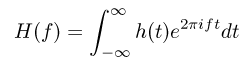 (2)
(2)
where t is in
seconds and f is in cycles per second.
In a measured dataset the function h(t) is not continues, but represents the
value of the function at discreet and here uniform time intervals,  . The function in time is then
represented by
. The function in time is then
represented by where n
goes from 0 to N. With such a representation there is a
maximum frequency that can be represented, namely
where n
goes from 0 to N. With such a representation there is a
maximum frequency that can be represented, namely  , representing the Nyquist frequency. This implies
that the shortest wavelength is represented by only two data points. For
frequencies higher than this there is no unambiguous representation. Instead
these will be seen as waves with longer wavelength and therefore be responsible
for giving a wrong Fourier transform. This phenomena is knows as aliasing and is
shown in the image below:
, representing the Nyquist frequency. This implies
that the shortest wavelength is represented by only two data points. For
frequencies higher than this there is no unambiguous representation. Instead
these will be seen as waves with longer wavelength and therefore be responsible
for giving a wrong Fourier transform. This phenomena is knows as aliasing and is
shown in the image below:
This image also shows how
different samplings of a sinusoidal function looks, and how a too high frequency
wave gives rise to a false low frequency wave representation. This implies that
if the data are limited in frequency such that highest frequency is less than
the Nyquist frequency, then the discreet Fourier representation is exact. When
this is not the case, then additional power to various frequencies are obtained
through the aliasing seen above and a wrong answer is obtained. From a frequency
point of view, these are the "allowed" frequencies that can be obtained:
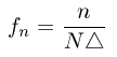
, where
n
goes from
-N/2 to
N/2.
Under these conditions it is
possible to rewrite the expressions in eq.(1) and eq.(2) as
 (3)
(3)
and
 (4)
(4)
In this part of the exercise, you have to write a code that:
- Read the data from a file specified at run time. Assume the data files for
the cases below are written in ASCII format. The first line indicate the
length of the 1D data array to follow. This assumes the time difference
between the data point is uniform and therefore uninteresting as it only
represents a scaling factor in the analysis.
- For the initial testing, use the small data set 'data.dat'. This is a
specially constructed data set where the imposed wavenumbers are well
defined.
- The smart thing is to use allocatable arrays to store all the relevant
data.
- Make a simple Fourier transform using at first eq.(4).
- Notice that H(f) is a complex variable even when h is real.
- Save the functions f and H(f) in a file for later plotting with gnuplot --
requires three columns of data -- "time", f, |H(f)|. Where time is just a
running number starting at 1.
- From a few lines above eq.(4) you notice that the sum goes from -N/2 to
N/2. This indicates that there are N+1 values in H. This is due to the
symmetry, where the central element contains the constant value and
symmetrically on either side of this are two real amplitude values for the
given frequency. The correct amplitude of the given wavelength is obtained
by summing these two values
- From H(f) make the inverse transform to determine h using eq.(3).
- Notice, there is only a sign difference between eq.(3) and eq.(4) -- not
taking into account the normalisation. This makes it simple to use the same
routine when including the sign as an input. Only the scaling has to be
applied to the result after returning from the routine. or possible be build
into the routine...
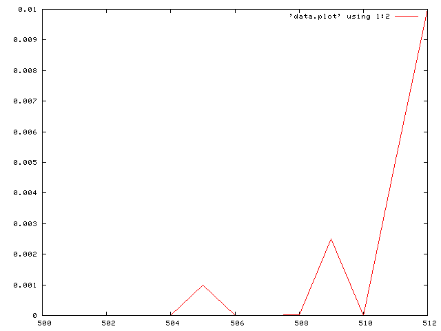
The figure shows the
amplitudes of the wavelengths that are included in the data.dat representation.
Plotting the full data set, you will only see a single value different from
zero, namely entry 513 that represents the mean value of g. This plot shows that
only three different wavelengths are represented in the data set.
Use
your program and data.dat to reproduce the graph above.
For large data set it can take quit some time to compute the Fourier
transform. Just to show you that FFT is much faster, and provides you with the
same result, you are going to change the previous simple FT method to the FFT
method given in Numerical recipes. It will not take long as it is all prepared
for in the Makefile. There are a few issues that have to be changed relative
your previous program:
- You only need one real array to contain both the initial data and the fft
- To call the FFT routine you need to include:
- use realft
- call realft_sp(ff,1)
- call realft_sp(ff,-1)
- ff represents the data and +/-1 the direction of the fft operation as
before.
- Again the scaling needs to be applied to give the correct answer
- First time multiply the result with 1/ndata.
- second time divide with 2.
Compare the time between the FT and the FFT version by using the Unix
command time.
$ time a.out < in.dat
where in.dat
contains the input information to the program you would otherwise type in by
hand (use man to check the information time provides).
To easily
see the difference, there are a number of data files in the directory
grav. They are called "dat.*.fft" where * goes from 0-10. The size of the
data increases with decreasing number. Try to time both the ft and the fft
version of the code using these data, starting with the small data sets. As you
will very soon realise, the ft version takes to long time, so DO NOT set it
running for more than a few minutes before you stop increasing the data size...
Save the effective run times for the two methods as a function of N (first entry
in the files) and plot the result with gnuplot, call the image timing.png
(use log scales). To test that the scaling I hinted earlier is not totally out
of the blue, include two well fitting lines that represernts the scaling of the
computation time for the two cases.
$Id: index.php,v 1.17 2009/10/06 07:29:58 kg Exp $ kg@astro.ku.dk
