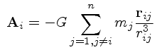
 (1) (1)
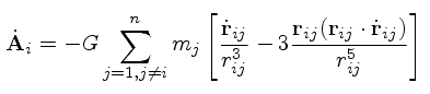
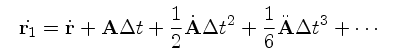
 (3)
(3) and
and 
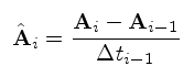
 (4)
(4) (5)
(5) (6)
(6) (7)
(7) (8)
(8) (9)
(9) (10)
(10)| parameter/object |
A |
B |
C |
| x |
1 |
-2 |
1 |
| y |
3 |
-1 |
-1 |
| z |
0 |
0 |
0 |
| vx |
0 |
0 |
0 |
| vy |
0 |
0 |
0 |
| vz |
0 |
0 |
0 |
| mass |
3 |
4 |
5 |
|
|
|
|